News

Azzolin et al. introduced the idea of 'pacing at the end of the refractory period' (PEERP) in 2021 as described in the corresponding paper. In the following, we provide a more technical description how PEERP is peerping and introduce a couple of improvements.

In the original PEERP implementation, several values were hardcoded. We keep these values for compatibility and made them changeable in PEERP_config.py. The corresponding variable names are written in ALL CAPS in the following.

TLDR Changes

• Fixed bug in reentry detection where only one point instead of the whole ring was used to look for an activation
• Added LAT based analysis for ERP propagation (see section “Stimulus propagation analysis”)
• Major refactoring to make changes easier and added plenty of debugging options

Algorithm

The main idea is to start with a prepacing of e.g. 5 S1 beats (e.g. from the sinus node) and then add stimuli at the end of the effective refractory period (ERP) after the last S1 stimulus. If the S2 stimulus does not induce a reentry, the algorithm adds an S3 stimulus after the ERP of the S2 stimulus. This is repeated until a reentry is induced or the maximum number of iterations (args.max_n_beats_PEERP, see flow chart) is reached.

PEERP can be split into two parts:

Binary search to identify the effective refractory period (ERP)

As the ERP can vary between different positions in the tissue, it has to be identified on a per-point basis. Therefore, first a search window is defined based on a priori knowledge of physiologically possible ERP values. This is for the first S2 stimulus centered on action potential duration (APD) and activation time (ACT, S2=ACT+APD). For all additional beats (S3-SN), it is defined based on the last ACT. To do so, first the lower bound of the search window is set as the next available saved state after the last stimulus, which is at least 60ms after this stimulus. Starting from this lower bound, the new stimulus is defined as lower_bound+80ms (OFFSET_S2_NEW_BEAT). The upper bound is then defined by S2+40ms (OFFSET_UPPPER_BOUND_NEW_BEAT). To find the ERP, a binary bisection search is applied. We define the end of ERP by the first propagating stimulus. Therefore, we test if a stimulus set at the current stimulus time propagates.

Stimulus propagation analysis

In the previous version, successful propagation was defined as a maximum transmembrane voltage greater than -50mV (M2_THRESHOLD) in a ring (from 2 to 3 times the stimulus size (args.stim_size)) around the stimulation point. However, two stimuli can be shortly after one another. Combined with slow conduction velocities and fibrotic regions, this can lead to late activation times. In these scenarios, the initial implementation of propagation analysis can misclassify propagation by detecting activation from a previous stimulus (false positive; see Fig. 1). This misclassification could lead to an ERP search converging to the fixed set lower bound in the initial implementation, reducing the PEERP algorithm to a rapid pacing algorithm with an S2 period of 120ms. To fix this issue, we compare to the previous propagation based on observed local activation times (LATs). For this, we define three conditions for elements in the modified detection ring:

1. Points have to be in the detection ring \(2*stim_{size} \le r \le 3 * stim_{size}\), with \(r\) being the distance between the checked point and the stimulated point;
2. LATs have to be after the stimulus;
3. LATs cannot be later than 60ms after the stimulus, as we only simulate for 60ms;
4. The difference between the LAT with the stimulus and without it has to be greater than 10ms (see Fig. 2).

The third condition assures that the new stimulus did indeed influence the LAT and the activation is not based on an old stimulus. Because simulation for prepacing and between different beats lasts longer than the new stimulus, we can use the LATs from these simulations, so no extra simulations are needed for this evaluation.

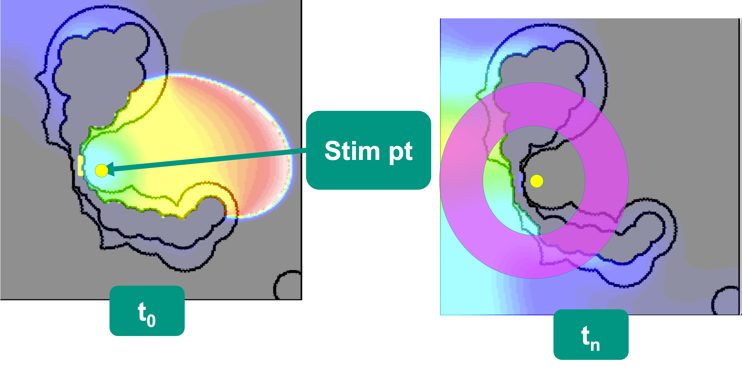
Fig. 1: Example of wrong classification in the initial implementation. Because the previous stimulus takes too long around the large fibrotic patch, the new stimulus is detected as capturing (non-refractory) because the left part of the ring is activated regardless of what happens at the stimulus point.

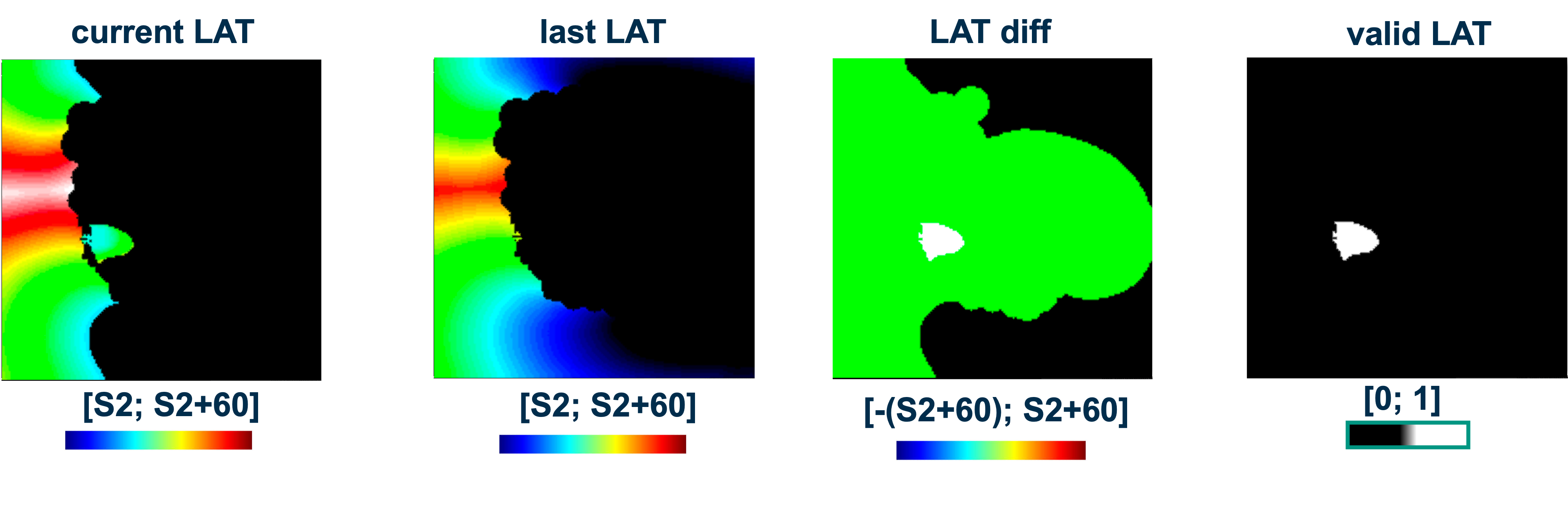
Fig. 2: LAT based filtering. The valid LAT is calculated out of the LAT difference (difference greater than 10ms, condition 4) and the current LAT after the new stimulus (condition 2 and 3). Green areas in the LAT diff picture correspond to a difference of 0, white areas to a positive difference (LAT with the new stimulus but not without this stimulus), black areas to negative difference (no LAT with new stimulus, LAT without the new stimulus)

Reentry detection

The detection of reentries follows a two-stage approach. In the first stage, we simulate for 400ms (REENTRY_SEARCH_STIM_DURATION) after the last stimulus and evaluate the last 100ms (REENTRY_EVALUATION_PERIOD) in the detection ring to check if the maximum transmembrane voltage is above -50mV (M2_THRESHOLD). If this is the case, we save the activation in jobID+saved.txt; if not, we directly go to the next beat. To see if this initial reentry is sustained, we simulate for one second (PERSISTENT_REENTRY_SEARCH_SIM_DURATION) after the last stimulus. If we still have an activation in the ring after this second stimulus, we classify this stimulus as inducing a reentry and store it in reentry.txt as well as the igb file in reentry_POINT_ID_at_S2_STIMTIME. If no reentry is found, we look for the next possible beat after the ERP or go to the next point depending on the number of beats tried already (args.max_n_beats_PEERP).

Debugging

For debugging, PEERP offers multiple options at different levels of detail.

Debugging flag off (--debug 0)

• PEERP_log.log This file contains all command line outputs of the PEERP algorithm (no openCARP, meshtool, etc.). This contains errors, the current stim point's coordinates, the current S2 time, refractory/non-refractory information, execution times etc.
• converge_eb_stats.csv This file gives information about the ERP search phase of the PEERP algorithm. It saves the lower/upper bound of the ERP search window as well as execution times and the voltage leading to the search decision.

Debugging flag on (--debug 1)

The resulting files in jobID/point_n/beat_m/ are:

• vm_it_I.igb: transmembrane voltage for the i-th iteration of the ERP search
• nodes_to_check_it_I: valid nodes for refractoriness assessment based on LAT filtering
• lastLATs.dat: last activation times without the current stimulus
• currentLATs.dat: activation times with the current stimulus
• latDifferences: currentLAT-lastLATs
• valid_LATs: binary result/mask of LAT filtering

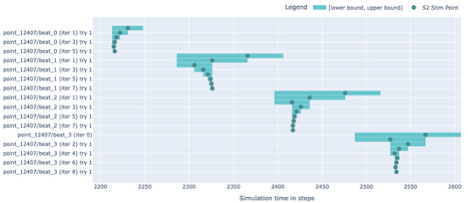
Fig. 3: Visualization of converge_EB_stats.csv. Iteration of the ERP search algorithm for 4 stimuli (S2-S5). The bars represent the current search window, while the dots show the used stimulus time point. We can also see the APD and ACT-dependent shorter first search window, while the other windows have a fixed size of 120 ms.

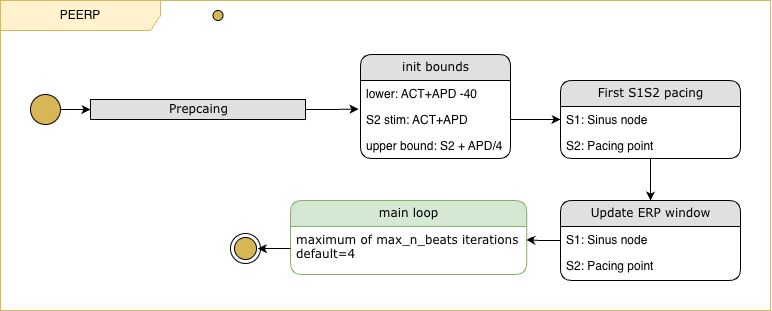
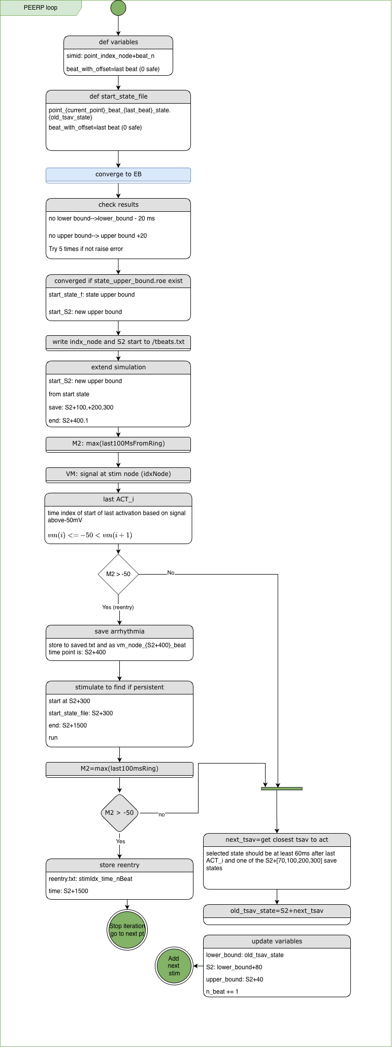
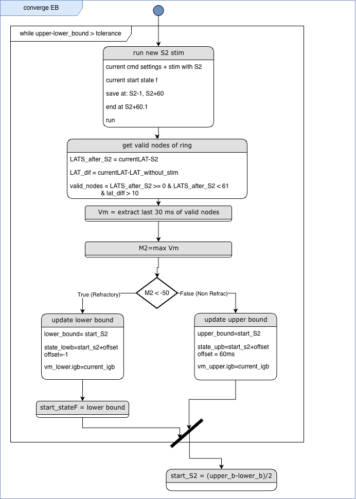
Flowcharts