openCARP examples
These examples are intended to showcase most openCARP features in a hands-on way. The scripts are designed as mini-experiments, which can also serve as basic building blocks for more complex experiments. This example can be a good starting point to base your own experiment on. If you are completely new to openCARP, the tutorials are ideal for onboarding.
All executable examples are coded up in carputils to facilitate an easy execution of all experiments including mesh generation, pre- and post-processing without complex command line interactions. If you prefer running the core simulation directly using bare-metal openCARP, passing the --dry-run option will output all subprocess commands that would be executed by the carputils script.
Do you want to improve the existing examples or contribute an additional one? We provide instructions in the experiments repository.
Intended use
Most examples can be run by simply copying the command from the corresponding example web page. It is recommended to inspect the generated command lines to understand what the simulation looks like in the plain command line by adding the option --dry to the run script command line. You can download the examples from our repository.
Available examples
We provide examples covering the following use case classes:
- Single cell electrophysiology
- Monodomain and bidomain tissue models
- Eikonal-based tissue models
- Simplified Kirchhoff network models
- Extracellular-intracellular-membrane (EMI) model
- Visualization
- Pre- and post-processing
Electrophysiology in single cell
The following examples illustrate how single cell modeling is performed using the tool bench. Additionally you learn how to integrate a single cell model from CellML into our library limpet using the math language EasyML
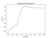
Basic single cell EP and limit cycle
This example introduces the basic steps of running electrophysiological simulations in an isolated myocyte using bench and limpetgui.
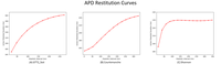
APD restitution
Action potenital duration (APD) restitution example in a single cell. As pacing frequency is increased, APD shortens.
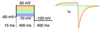
Voltage clamp
This example explains the basic usage of bench for performing voltage clamp experiments.
EasyML to C code
This example explains the basics of using the code generation tool limpet_fe.py for generating ODE solver code for models of cellular dynamics. It also covers the creation of new models as a dynamic library.
EasyML basics
More information about the cell model math format EasyML.
Electromechanical coupling
Couple an electrophysiological cell model to a tension model.

Convert CellML to EasyML (.model)
Here you learn how to import CellML data into openCARP and what problems might occur during this process.

Convert EasyML (.model) to CellML
Learn how to convert your .model file (EasyML) to CellML.
Parallel single-cell simulations
See how to execute single-cell simulations in parallel and build populations of models.
Monodomain and bidomain tissue models
These examples inform about basic steps in developing tissue simulations based on the monodomain and bidomain models
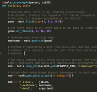
Simple carputils example
This is not a real example but more of a template to base your own experiment on. It covers mesh generation, monodomain simulation and local activation time extraction during postprocessing.
Basic tissue EP: AP propagation
This example introduces to the basics of using the openCARP executable for simulating EP at the tissue and organ scale.
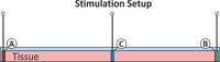
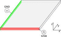
Extracellular stimulation
In this example you learn how to stimulate a tissue from the extracellular space.
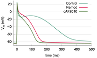
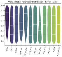
Ionic model parameter adjustment to match APD
This example demonstrates how to adjust ionic model parameters to generate a specific action potential duration in your simulations.
Tuning conduction velocity
This example introduces the background for the relationship between conduction velocity and tissue conductivity.
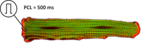
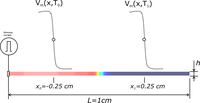
Limit cycle initialization; cell to tissue state transfer
This example demonstrates how to initialize a cardiac tissue with state variables obtained from a single-cell stimulation.
Model parameter adjustment to match wavelength
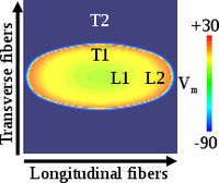
This example demonstrates how to adjust parameters in tissue simulations to match experimental data for conduction velocity, APD, and wavelength.
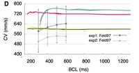
Conduction velocity restitution
This example demonstrates how to compute conduction velocity (CV) restitution in cardiac tissue.
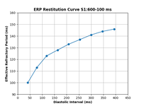
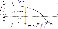
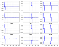
ERP restitution
This example shows how to calculate the effective refractory period (ERP) for a given combination of ionic conductances in a tissue slab using an S1S2 pacing protocol. An ERP restitution curve can also be plotted, if desired by the user.
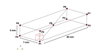
Niederer et al. benchmark: numerical discretization
This example replicates the Niederer et al. benchmark and illustrates effects of some numerical settings including temporal and spatial discretization.
Region tagging
Regions are used to manage the assignment of heterogeneous tissue properties. This example explains the different approches of how regions can be defined.
Heterogeneity: conductivity regions
This example details how to assign different conductivities to different parts of a simulated tissue slice using region-wise tagging.
Heterogeneity: ionic model regions
This example details how to assign different single cell dynamics to different parts of a simulated tissue slice using region-wise tagging.
Heterogeneities: regions vs. gradiensts (nodal adjustment)
This example introduces the concepts of region-based and gradient-based heterogeneities for assigning spatially varying properties.
Heterogeneities: smooth gradients via nodal adjustments of ionic model parameters
This example details how to assign a gradient of single cell properties using the adjustments interface.

Output spatio-temporal state variable distributions
This example details how to output the values of state variables over time during a simulation.
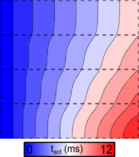
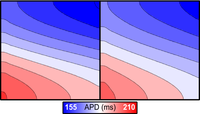
Electrical mapping (LAT)
This example demonstrates how to compute local activation times (LATs) and action potential durations (APDs) of cells in a cardiac tissue during the simulation rather than during postprocessing.
Extracellular potentials and ECGs
This example explains the background of computing extracellular potentials and ECG using different techniques.
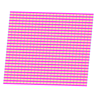
Periodic boundary conditions
Periodic boundary conditions connect the left edge of a sheet to the right, or the top to the bottom.

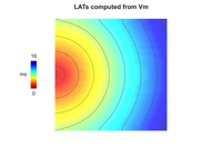
Local activation time
This example demonstrates how to compute local activation times (LATs) and action potential durations (APDs) of cells in a cardiac tissue
Lead field ECG
Lead field example showing how to compute the ECG lead field for a given source and sensor configuration.
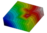
Laplace solutions
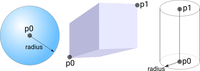
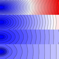
Computing Laplace-Dirichlet maps provide an elegant tool for describing the distance between defined boundaries.
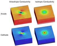
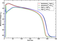
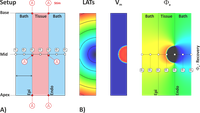
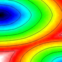
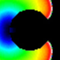
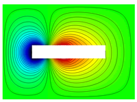
Unequal anisotropy effects
Unequal anisotropy ratios in bidomain simulations can be responsible for the formation of unexpectedly complex polarization patterns.
Parameter sweeps
This example shows how to use polling files to sweep parameters.
Reentry induction protocols
This example shows the influence of different induction protocol on reentry initiation and maintenance.

ForCEPSS: VARP Protocol
This example demonstrates the usage of ForCEPSS implementation of the VARP (Virtual Arrhythmia Risk Predictor) protocols in the context of cardiac electrophysiology simulations.

Checkpointing, restarting & sentinel (quiescence watchdog)
This example demonstrates two ways of setting checkpoints, restarting from checkpoints and automatic simulation termination based on a LAT watchdog (sentinel).
Eikonal-based tissue models
These examples inform about basic steps in developing tissue simulations based on the eikonal, reaction-eikonal and DREAM models
Eikonal model
This example demonstrates how to set up and use the eikonal model.
Reaction-Eikonal Model
This example shows how to run reaction-eikonal simulations with (RE+) and without diffusion current (RE-).
Diffusion Reaction Eikonal Alternant Model - Pacing
This example demonstrates and explores pacing behavior while using the DREAM.
Diffusion Reaction Eikonal Alternant Model - Reentry
This example demonstrates how to set up and use the DREAM to simulate reentries.
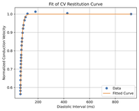
Fitting CV restitution
This example shows how to find the parameters for CV restitution to use DREAM with other ionic models.
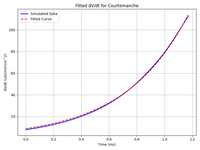
Fitting foot current parameters
This example shows how to find the parameters for Ifoot to run reaction-eikonal with other ionic models.
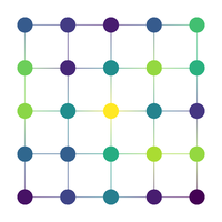
Simplified Kirchhoff network models
These examples demonstrate the use of simplified Kirchhoff network models
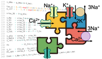
The extracellular-membrane-intracellular (EMI) model
These examples demonstrate the use of the EMI model
EMI basics
Introduces EMI in openCARP on two gap-junction-coupled cells: .intra/.extra mesh anatomy, gen_physics_opts, ConductivityRegionEMI, imp_region_emi, and per-cell heterogeneity — with the carputils parameter strings each call generates.
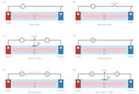
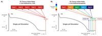
EMI stimulation modes
Demonstrates EMI stimulus circuit types on a 10-cell cardiomyocyte chain, grouped by domain: extracellular voltage and current sources (clamped, balanced, open-loop), an intracellular sharp microelectrode, and direct transmembrane stimulation.
Visualization
Learn how to use the visualization tools LimpetGUI for single cell results as well as Meshalyzer and ParaView for tissue results
limpetGUI
limpetGUI is a simple tool for visualizing traces output generated by bench.

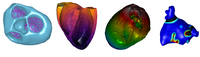
Meshalyzer
meshalyzer is a 4D visualization tool for openCARP allowing interactions to investigate data.
Meshalyzer: Advanced features
A few advanced features of meshalyzer are explained here to make life simpler.
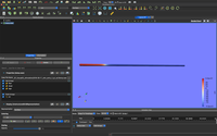
Paraview visualization
This is an example to visualize the time series of a simple tissue geometry in ParaView.
Pre- and post-processing
Learn how to use the meshing tools and how to postprocess igb files