Basic usage of single cell tool bench - Limit cycle experiments

See code in GitLab.
Author: Gernot Plank gernot.plank@medunigraz.at

cd ${TUTORIALS}/01_EP_single_cell/01_basic_bench 

Modeling EP at the cellular level

This tutorial introduces the basic steps of setting up EP simulations in an isolated myocytes. A more detailed account on modeling EP at the cellular scale and the single cell EP simulation tool bench is given in chapters 5 and 8 of the openCARP manual. Before starting we recommend therefore to look up the basic command line options there. In this introductory tutorial, we focus on simple pacing protocols for finding a stable limit cycle. 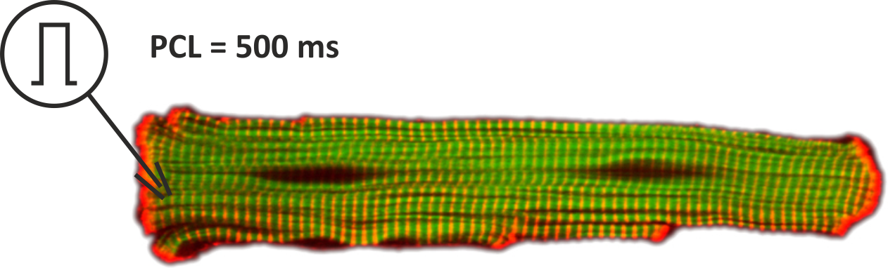We model an isolated myocyte, which we stimulate using an electrode for intracellular current injection. The setup is shown in _fig-single-cell-EP.

Experimental Parameters

The following parameters are exposed to steer the experiment:

--EP {tenTusscherPanfilov, DrouhardRoberge, OHara}        pick human EP model (default is tenTusscherPanfilov)

--EP-par EP_PAR       provide a parameter modification string (default is '')

--init INIT           pick state variable initialization file (default is none)

--duration DURATION   pick duration of experiment (default is 500 ms)

--bcl BCL             pick basic cycle length (default is 500 ms)

--visualize           plots the myocyte action potential

--overlay             overlays the action potential or specified variables of several
                      experiments in the same plot

--vis_var VIS_VAR     specified the variables that you want to visualize (default is V)

Each experiment stores the state of myocyte and myofilament in the current directory in a file to be used as initial state vector in subsequent experiments.

Limit cycle experiments

Background on the computaiton of limit cycles is found in the limit cycle section of the manual. Briefly, models of cellular dynamics are virtually never used with the values given for the initial state vector. Rather, cells are based to a given limit cycle to approximate the experimental conditions one is interested in. The state of the cell can be frozen at any given instant in time and this state can be reused then in subsequent simulations as initial state vector. In the following experiments the procedures for finding an initial state vector for a given model and a given basic cycle length are elucidated. To run the experiments of this tutorial change directories as follows:

cd ${TUTORIALS}/01_EP_single_cell/01_basic_bench 

To see all the exposed parameters itemized above in experimental parameters section.

run

./run.py --help

Experiment exp01 (short pacing protocol)

We start with pacing the tenTusscherPanfilov human myocycte model at a pacing cycle length of 500 ms for a duration of 5 seconds (5000 msecs).

./run.py --EP tenTusscherPanfilov --duration 5000 --bcl 500 --ID exp01 --visualize --vis_var ICaL INa IK1

You will get an overview of current traces of the model.

Experiment exp02 (limit cycle pacing protocol)

In experiment exp01 we observed that the state variables of the model did not stabilize at a stable limit cycle. We increase therefore the duration of our pacing protocol to 20 seconds (20000 msecs).

./run.py --EP tenTusscherPanfilov --duration 20000 --bcl 500 --ID exp02 --visualize

At the end of the pacing protocol the initial state vector is saved in the file exp02_tenTusscherPanfilov_bcl_500_ms_dur_20000_ms.sv.

-85.0922            # Vm
-                   # Lambda
-                   # delLambda
-                   # Tension
-                   # Ke
-                   # Nae
-                   # Cae
0.00312354          # Iion
-                   # tension_component
-                   # illum
tenTusscherPanfilov
3.9033              # CaSR
0.000391138         # CaSS
0.135498            # Cai
3.43519e-05         # D
0.726548            # F
0.958436            # F2
0.995449            # FCaSS
3.98e-05            # GCaL
0.153               # GKr
0.392               # GKs
0.294               # Gto
0.740339            # H
0.669782            # J
137.333             # Ki
0.0017662           # M
7.96972             # Nai
2.47788e-08         # R
0.904552            # R_
0.999972            # S
0.0171519           # Xr1
0.46972             # Xr2
0.01471             # Xs

Ionic model parameter modification experiments

Model behavior can be modified by providing parameter modification string through --imp-par. Modifications strings are of the following form:

param[+|-|/|*|=][+|-]###[.[###][e|E[-|+]###][\%]

where param is the name of the paramter one wants to modify such as, for instance, the peak conductivity of the sodium channel, GNa. Not all parameters of ionic models are exposed for modification, but a list of those which are can be retrieved for each model using imp-info. As an example, let's assume we are interested in specializing a generic human ventricular myocyte based on the ten Tusscher-Panfilov model to match the cellular dynamics of myocytes as they are found in the halo around an infract, i.e.in the peri-infarct zone (PZ). In the PZ various currents are downregulated. Patch-clamp studies of cells harvested from the peri-infract zone have reported a 62% reduction in peak sodium current, 69% reduction in L-type calcium current and a reduction of 70% and 80% in potassium currents \(I_{\mathrm {Kr}}\) and \(I_{\mathrm {K1}}\), respectively. In the model these modifcations are implemented by altering the peak conductivities of the respective currents as follows:

# both modification strings yield the same results
--imp-par="GNa-62%,GCaL-69%,GKr-70%,GK1-80%"

# or
--imp-par="GNa*0.38,GCaL*0.31,GKr*0.3,GK1*0.2"

In this experiment EP model parameters strings can be passed in using the --EP-par which expects parameter strings as input. The results of such modifications are illustrated in the following experiments.

Experiment exp03 (short pacing with modified myocyte)

In this experiment we modify the behavior of a tenTusscherPanfilov myocyte to match experimental observations of myocytes harvested from peri-infarct zones in humans. Initially, we simulated one cycle only to observe the effect of parameter modifications relative to the baseline tenTusscherPanfilov model. The reference traces are passed in and you can compare the experiment output.

./run.py --EP tenTusscherPanfilov --duration 5000 --bcl 500 --ID exp03 --EP-par "GNa-62%,GCaL-69%,GKr-70%,GK1-80%"             --visualize --overlay

Make sure that the parameter modification string is correctly interpreted by bench by inspecting the output log:

./run.py --EP tenTusscherPanfilov --duration 500 --bcl 5000 --ID test --EP-par "GNa-62%,GCaL-69%,GKr-70%,GK1-80%"


... 
Ionic model: tenTusscherPanfilov
     GNa                  modifier: -62%            value: 5.63844
     GCaL                 modifier: -69%            value: 1.2338e-05
     GKr                  modifier: -70%            value: 0.0459
     GK1                  modifier: -80%            value: 1.081
...

Experiment exp04 (limit cycle pacing with modified myocyte)

We repeat exp03 as a limit cycle experiment now by pacing for 20 seconds (20000 msecs). State variable and current traces stored in the baseline experiment exp02 are used as a reference.

./run.py --EP tenTusscherPanfilov --duration 20000 --bcl 500 --ID exp04 --EP-par "GNa-62%,GCaL-69%,GKr-70%,GK1-80%"             --visualize --vis_var Cai

Visual comparison of the traces reveals that Calcium-cycling in the peri-infarct myocyte shows alternans. The difference in initial state vectors between baseline and peri-infarct myocyte stored at the end of the pacing protocol can be inspected with the meld or any other diff program of your choice.

meld exp02_tenTusscherPanfilov_bcl_500_ms_dur_20000_ms.sv exp04_tenTusscherPanfilov_bcl_500_ms_dur_20000_ms.sv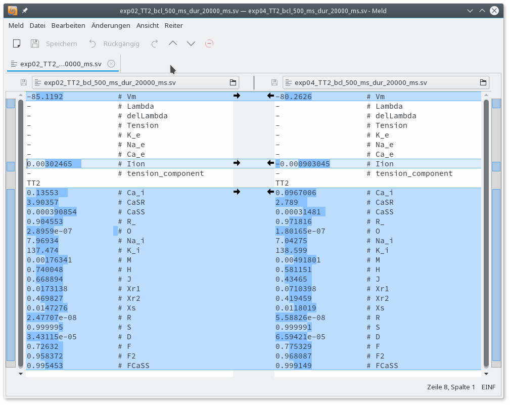

Recent questions tagged parameters, single_cell, models