Electromechanical coupling - single-cell stretcher
See code in GitLab.
Author: Gernot Plank gernot.plank@medunigraz.at and Christoph Augustin christoph.augustin@medunigraz.at
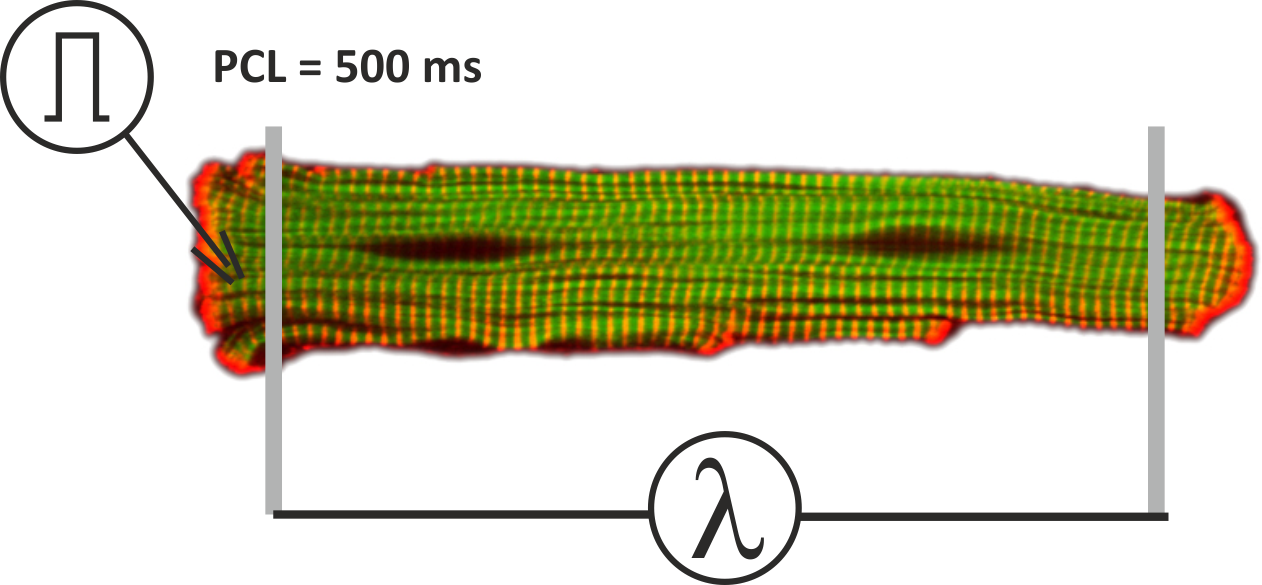
Single-cell electromechanics example
This example demonstrates how to set up and run single-cell electromechanical (EM) simulations using our bench tool.
We will couple electrophysiology (EP) models of cellular dynamics with myofilament models that generate active stress, mimicking real myocyte stretch experiments. Depending on the scientific question, different coupling schemes can be selected:
- Activation-based models simple, fast to simulate (parameters map to measurable outputs)
- Weakly coupled Ca-driven models tension depends on Ca transients but without feedback to EP
- Strongly coupled models bi-directional mechano-electric feedback (MEF), where mechanics affect EP
This example will guide you step by step through experiments, from initialization to reproducing published protocols.
To get started, navigate to the directory:
cd ${EXAMPLES}/01_EP_single_cell/06_EM_couplingExperimental parameters
The main command-line options are:
--experiment {active | passive}   # default: active
                                  # "passive" disables stimulation (resting myocyte)

--EP MODEL                        # electrophysiology model (default: tentusscherpanfilov)

--stress MODEL                    # stress model (default: stress_niederer11)

--stretch VALUE                   # prescribe constant fiber stretch (default: 1.0)

--init FILE                       # state initialization file (default: none)

--duration MS                     # experiment duration (default: 500 ms)

--bcl MS                          # basic cycle length (default: 500 ms)

--fs FILE                         # file with fiber stretch protocol (default: none)

--fsDot FILE                      # file with stretch velocity protocol (default: none)

--visualize                       # plot action potentials / tension traces

--overlay EXP                     # overlay traces from multiple experiments

--vis_var VARS                    # choose variables to plot (default depends on model)
Each experiment stores the final state of myocyte and myofilament in the current directory as a state vector file. These can be reused for initialization in subsequent experiments.
Tip: Always check that your simulation has reached a limit cycle before using the state for further experiments.
Activation-based active stress model
Activation-based models are well-suited for clinical EM studies, since their small parameter sets are easier to fit to measurable outputs such as peak pressure (\(\hat{P}\)) or maximum upstroke velocity (\(\mathrm{d}P/\mathrm{d}t_{\max}\)).
Here we use the simple stress_niederer11 model.
It generates length-dependent active tension transients using exponential
functions. This model has been applied in multiple studies
1
2
.
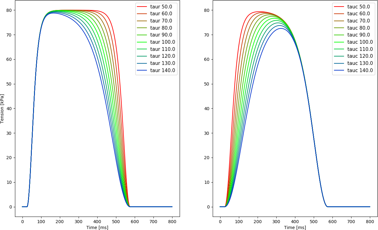
The shape of the active stress transient is given by
\[T_{\rm a} = T_{\rm peak} \, \phi \, \tanh^2 \left( \frac{t_{\rm s}}{\tau_{\rm c}} \right) \tanh^2 \left( \frac{t_\text{dur} - t_{\rm s}}{\tau_{\rm r}} \right), \qquad 0< t_{\rm s} < t_{\rm dur}{,}\]
with
\[\begin{aligned} \phi &= \tanh (\text{ld} (\lambda - \lambda_{\rm 0})){,} \nonumber \ \tau_{\rm c} &= \tau_{\rm c0} + \text{ld}_\text{up} (1 - \phi){,} \nonumber \ t_{\rm s} &= t - t_\text{act} - t_\text{emd}{,} \nonumber \end{aligned}\]
with the following parameters:
| Variable | Description |
|---|---|
| \(t_{\rm s}\) | Onset of contraction (ms) |
| \(\phi\) | Non-linear length-dependent function in which \(\lambda\) is the fiber stretch |
| \(\lambda_{\rm 0}\) | Fiber stretch with no tension generated |
| \(t_{\mathrm{emd}}\) | Electro-mechanical delay (ms) |
| \(T_{\mathrm{peak}}\) | Peak isometric tension (kPa) |
| \(t_{\mathrm{dur}}\) | Duration of tension generation (ms) |
| \(\tau_{\mathrm{c}}\) | Time constant of contraction (ms) |
| \(\tau_{\mathrm{c0}}\) | Baseline contraction time constant (ms) |
| \(ld_{\mathrm{up}}\) | Length-dependence of contraction time constant |
| \(\tau_{\mathrm{r}}\) | Time constant of relaxation (ms) |
| \(ld\) | Degree of length dependence |
| \(ld_{\mathrm{on}}\) | Flag to turn on/off length-dependence of active stress |
| \(t_{\mathrm{act}}\) | (ms), estimated from the action potential as the instant of crossing the \(V_{\rm m}\) threshold |
| \(V_{\rm m,thresh}\) | Transmembrane voltage (mV) threshold used for detecting \(t_{\mathrm{act}}\) |
.
Experiment exp01 - basic EM coupling
We start with coupling the Niederer tanh stress model with the tentusscherpanfilov human myocyte model:
./run.py --EP tentusscherpanfilov --stress stress_niederer11 \
         --duration 2000 --bcl 500 --ID exp01 \
         --visualize --vis_var V Cai Tension
Expected result: You should see action potential traces and Ca transients with visible beat-to-beat variation. In the phenomenological stress model, tension transients are calcium-independent and identical from the first beat onward.
Experiment exp02 - pacing to limit cycle
As the tentusscherpanfilov is not at a limit cycle, we pace the model for 50 seconds
./run.py --EP tentusscherpanfilov --stress stress_niederer11 \
         --duration 50000 --bcl 500 --ID exp02 \
         --visualize --vis_var V Cai Tension
Expected result: You should see action potential traces and Ca transients converging to a limit cycle.
Note: In exp02 the states of myocyte and myofilament model are stored at the very end of
the experiment at t 50000 ms in the file
exp02_tentusscherpanfilov_stress_niederer11_bcl_500_ms_dur_50000_ms.sv.
Experiment exp03 - confirm limit cycle
Using the state of the myocyte stored in the file
exp02_tentusscherpanfilov_stress_niederer11_bcl_500_ms_dur_50000_ms.sv in exp02
we confirm that the trajectories are close to a limit cycle:
./run.py --EP tentusscherpanfilov --stress stress_niederer11 \
         --duration 1000 --bcl 500 --ID exp03 \
         --init exp02/exp02_tentusscherpanfilov_stress_niederer11_bcl_500_ms_dur_50000_ms.sv \
         --visualize --vis_var V Cai Tension
Expected result: You should see stable action potential traces, Ca transients, and a periodic tension transient with no visible variation from the first to the second beat.
Experiment exp04 - length-dependence (shortening)
To ensure that length-dependence of active tension is working as expected, we re-run the experiment at a shorter cell length by setting the fiber stretch \(\lambda=0.85\) and compare with the traces generated in exp03 at the reference cell stretch \(\lambda=1.0\).
./run.py --EP tentusscherpanfilov --stress stress_niederer11 \
         --duration 1000 --bcl 500 --ID exp04 --stretch 0.85 \
         --init exp02/exp02_tentusscherpanfilov_stress_niederer11_bcl_500_ms_dur_50000_ms.sv \
         --overlay exp03 --visualize --vis_var V Cai Lambda Tension
Expected result: Reduced sarcomere length (\(\lambda=0.85\)) produces lower peak tension, while AP and Ca remain unchanged (activation-based model has no MEF).
Experiment exp05 - length-dependence (myocycte stretching)
Re-run experiment exp04, but at a stretched cell length by setting the fiber stretch \(\lambda=1.15\) and compare again with the traces generated in exp03 at the reference cell stretch \(\lambda=1.0\).
./run.py --EP tentusscherpanfilov --stress stress_niederer11 \
         --duration 1000 --bcl 500 --ID exp05 --stretch 1.15 \
         --init exp02/exp02_tentusscherpanfilov_stress_niederer11_bcl_500_ms_dur_50000_ms.sv \
         --overlay exp03 --visualize --vis_var V Cai Lambda Tension
Expected result: Increased sarcomere length (\(\lambda=1.15\)) produces higher peak tension, while AP and Ca remain unchanged (activation-based model has no MEF).
Weakly coupled calcium-driven active stress model
Weakly coupled models such as stress_land17 capture the dependence of
tension on Ca transients
3
4
, but do not feed back
mechanical effects to electrophysiology. They are more physiological than purely
activation-based models but are harder to calibrate to given data.
| Variable | Description |
|---|---|
| \(T_{\rm {ref}}\) | Reference tension (kPa) | | |
| \(Ca_{\rm {50ref}}\) | Calcium sensitivity at resting sarcomere length | | |
| \(TRPN_{\rm {50}}\) | Troponin C sensitivity | | |
| \(n_{\rm {TRPN}}\) | Hill coefficient for cooperative binding of Calcium to Troponin C | | |
| \(k_{\rm {TRPN}}\) | Unbinding rate of Calcium from Troponin C | | |
| \(n_{\rm {xb}}\) | Hill coefficient for cooperative crossbridge action | | |
|
|
| \(\beta_{\rm {0}}\) | magnitude of filament overlap effects | | |
| \(\beta_{\rm {1}}\) | magnitude of length-dependent activation effects | | |
Experiment exp06 - pacing to limit cycle for a physiological model
As before with the Niederer tanh stress model, we pace the model for 50 seconds at a resting length of \(\lambda=1.\) to arrive at a limit cycle.
./run.py --EP tentusscherpanfilov --stress stress_land17 --duration 50000 --bcl 500 --ID exp06 --visualizeExpected result: Tension now depends directly on Ca transient amplitude and timing. All plotted values should converge to a limit cycle.
Note: In contrast to the Niederer tanh stress model (exp02),
the tension transients for the physiological Land stress model vary over the beats
due to their dependence on calcium concentration.
In exp06 the states of myocyte and myofilament model are stored at the very end of the
experiment at t 50000 ms in the file exp06/exp06_tentusscherpanfilov_stress_land17_bcl_500_ms_dur_50000_ms.sv.
Experiment exp07 - confirm limit cycle
Using the state of the myocyte stored in the
file exp06/exp06_tentusscherpanfilov_stress_land17_bcl_500_ms_dur_50000_ms.sv in exp06
we confirm now that your trajectories are close to a limit cycle for the
given bcl and stretch we run
./run.py --EP tentusscherpanfilov --stress stress_land17 --duration 1000 --bcl 500 --ID exp07 \
         --stretch 1.0 --init exp06/exp06_tentusscherpanfilov_stress_land17_bcl_500_ms_dur_50000_ms.sv \
         --visualize
Expected result: You should see stable action potential traces, Ca transients, and a periodic tension transient with little variation from the first to the second beat.
Experiment exp08 - length-dependence (myocycte shortening)
To verify that the Land model in combination with the tentusscherpanfilov human ventricular myocyte models produces reasonable tensions over the physiological stretch range from \(\lambda=0.85\) up to \(\lambda=1.15\) we run two cycles at with a shortened myocyte \(\lambda=0.85\).
./run.py --EP tentusscherpanfilov --stress stress_land17 --duration 1000 --bcl 500 \
         --ID exp08 --stretch 0.85 --init exp06/exp06_tentusscherpanfilov_stress_land17_bcl_500_ms_dur_50000_ms.sv \
         --overlay exp07 --visualize
Expected result: Shorter sarcomere length reduces Ca-dependent tension, AP and Ca remain unchanged.
Experiment exp09 - length-dependence (myocycte stretching)
Re-run experiment exp08, but at a stretched cell length by setting the fiber stretch \(\lambda=1.15\) and compare again with the traces stored in exp07 in the file exp07_traces.h5 at the reference cell stretch \(\lambda=1.0\).
./run.py --EP tentusscherpanfilov --stress stress_land17 --duration 1000 --bcl 500 \
         --ID exp09 --stretch 1.15 --init exp06/exp06_tentusscherpanfilov_stress_land17_bcl_500_ms_dur_50000_ms.sv \
         --overlay exp07 --visualize
Expected result: Sarcomere stretch increases Ca-dependent tension, AP and Ca remain unchanged.
Experiment exp10 - prescribed stretch profile
Force development depends on both, length \(\lambda\) and the velocity of
length change \(\dot{\lambda}\).
Increasing velocity \(\dot{\lambda}\) lowers the force produced by a myocyte
which produces the maximum force under isometric conditions, that is \(\dot{\lambda} = 0\).
To illustrate these two effects indpendently,
we re-run exp09 with a dynamic sawtooth loading protocol shown in fig-sawtooth-loading-ld,
but we keep the velocity at zero.
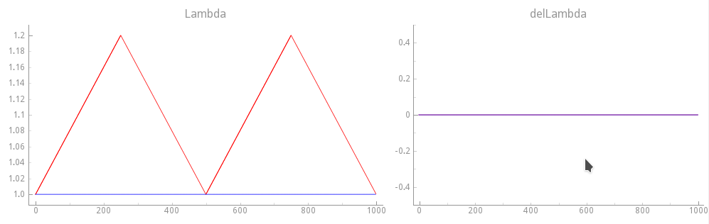
Note
This is artificial as we are altering \(\lambda(t)\) and \(\dot{\lambda}(t)\) independently.
./run.py --EP tentusscherpanfilov --stress stress_land17 --duration 1000 --bcl 500 \
         --ID exp10 --init exp06/exp06_tentusscherpanfilov_stress_land17_bcl_500_ms_dur_50000_ms.sv \
         --fs traces/lambda_sawtooth_200ms.dat \
         --overlay exp07 --visualize --vis_var Tension Lambda delLambda
Expected result: Sarcomere stretch increases Ca-dependent tension, AP and Ca remain unchanged.
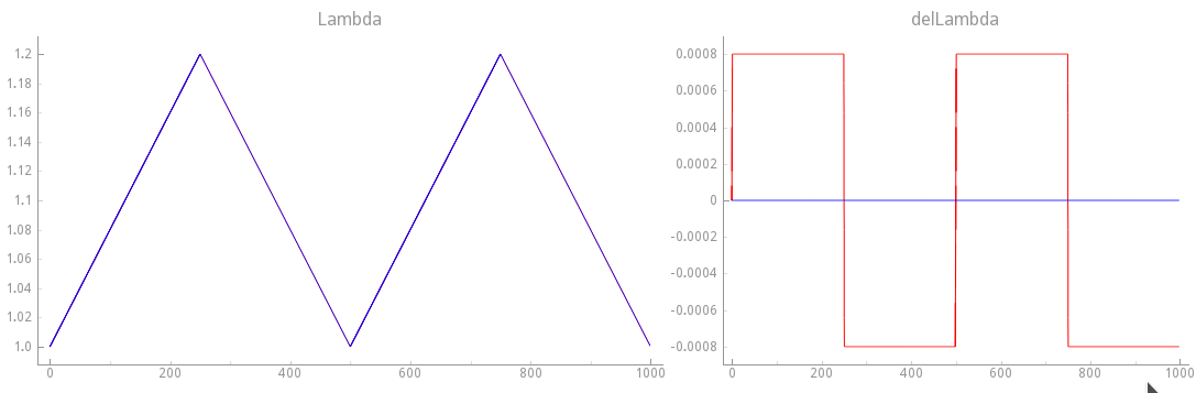
Experiment exp11 - force velocity relationship
In this experiment do not suppress velocity dependence anymore.
The mechanical loading protocol applied is the same as in exp10,
but with \(\dot{\lambda}(t) \neq 0\). The loading protocol is illustrated in
fig-sawtooth-loading-ld-vd.
./run.py --EP tentusscherpanfilov --stress stress_land17 --duration 1000 --bcl 500 \
         --ID exp11 --init exp06/exp06_tentusscherpanfilov_stress_land17_bcl_500_ms_dur_50000_ms.sv \
         --fs traces/lambda_sawtooth_200ms.dat --fsDot traces/dlambda_sawtooth_200ms.dat \
         --overlay exp10 --visualize --vis_var Tension Lambda delLambda
Expected result: When the fiber is lengthening, stretch-rate dependence increases tension.
Experiment exp12 - frequency dependence
./run.py --EP tentusscherpanfilov --stress stress_land17 --duration 50000 --bcl 1000 \
         --ID exp12 --overlay exp06 --visualize --vis_var V Cai Tension
Expected result: Shorter cycle length (faster pacing, exp06) increases intracellular Ca and tension.
Strongly coupled calcium-driven active stress model
Strongly coupled models include mechano-electric feedback (MEF), where stretch influences Ca handling and thus the AP itself. Here we use the Augustin model 5 , combining GPB EP 6 with Land–Niederer stress 7 .
Briefly, to allow for strong coupling, i.e., to account for length effects on the cytosolic calcium transient, modifications were implemented to both the GPB and the LN model. The equation governing the binding of calcium to the low affinity regulatory sites on Troponin in the myofilament model (see Eq.~(114) in the Appendix of 8 )
\[\begin{align} \frac{\mathrm{d}[\mathrm{TnC}_{\mathrm{L}}]}{\mathrm{d} t} = k_{\mathrm{on}_{\mathrm{TnC}_{\mathrm{L}}}}[\mathrm{Ca}_{\mathrm{i}}^{2+}] \left(\hat{B}_{\mathrm{TnC}_{\mathrm{L}}} -[\mathrm{TnC}_{\mathrm{L}}] \right) - k_{\mathrm{off}_{\mathrm{TnC}_{\mathrm{L}}}} [\mathrm{TnC}_{\mathrm{L}}] \nonumber \end{align}\]
is replaced by the analogous Eq.~(1) of the LN active stress model 9 , given as
\[\begin{align} \frac{\mathrm{d}\,\mathrm{TRPN}}{\mathrm{d} t} = k_{\mathrm{TRPN}} \left(\frac{[\mathrm{Ca}_{\mathrm{i}}^{2+}]} {[\mathrm{Ca}_{\mathrm{i}}^{2+}]_{\mathrm{T50}}(\lambda)} \right)^{n_\mathrm{TRPN}} \hspace{-2ex}\left(1 - \mathrm{TRPN}\right) - k_{\mathrm{TRPN}}\, \mathrm{TRPN}. \nonumber \end{align}\]
In the combined GPB+LN model, in the following called Augustin model, eq-Ca-Shannon is replaced by eq-LandTnC,
scaled by the total buffer concentration \(\hat{B}_{\mathrm{TnC}_{\mathrm{L}}}\)
assumed to be 70 \(\mathrm{\mu M/L}\) in the GPB model.
This scaling is necessary to correctly relate fractional occupancy,
used by the LN myofilament model, with the concentration of Troponin bound calcium,
used by the GPB model. Parameters of the GPB model were left unaltered whereas
parameters of the LN model were adapted to give human myocardium tension transients
when coupled to the GPB calcium transient
10
.
In single-cell experiments, both the unaltered GPB model and the combined Augustin model
were paced at a cycle length of 500 ms for a duration of 60 seconds.
In the combined Augustin model the stretch ratio was kept constant at \(\lambda=1.0\)
over the entire protocol.
In both models, all state variable transients were plotted over the entire pacing experiment
to ensure that the system had settled close to a stable limit cycle.
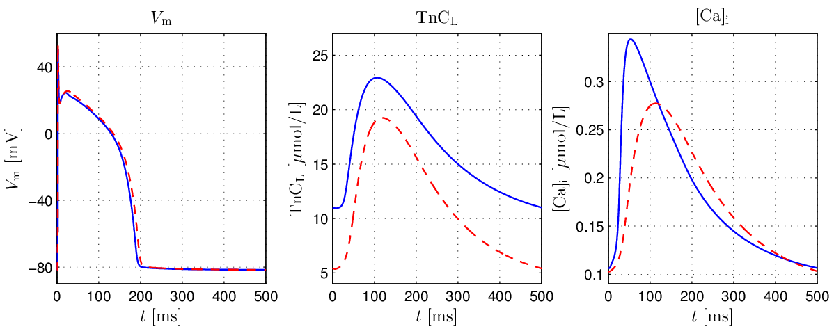
The effect of the altered Troponin buffering equation in the Augustin model
relative to the GPB model is illustrated in fig-GPB-LN-modified.
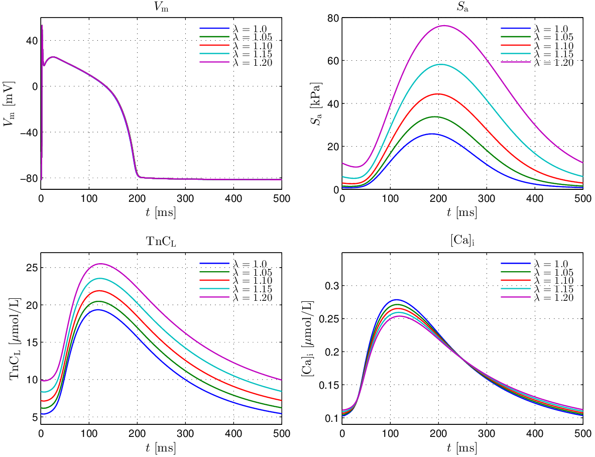
The effect of strong coupling in the Augustin model under fixed stretch conditions in the range
\(\lambda\in[1.0,1.2]\), with the same pacing protocol, is illustrated in
fig-GPB-length-dep.
Experiment exp13 - pacing to limit cycle
As before, we pace the model for 50 seconds at a resting length of \(\lambda=1.\) to arrive at a limit cycle.
./run.py --EP augustin --duration 50000 --bcl 1000 --ID exp13  \
         --visualize
Expected result: Action potential traces, Ca and tension transients converge to a limit cycle.
Experiment exp14 - confirm limit cycle
Using the state of the myocyte stored in the file
exp13/exp13_augustin_bcl_1000_ms_dur_20000_ms.sv in exp13
we confirm now that your trajectories are close to a limit cycle for the
given bcl and stretch we run
./run.py --EP augustin --duration 2000 --bcl 1000 --ID exp14 --stretch 1.0 \
         --init exp13/exp13_augustin_bcl_1000_ms_dur_50000_ms.sv \
         --visualize
Expected result: You should see stable action potential traces, Ca transients, and a periodic tension transient with little variation from the first to the second beat.
Experiment exp15 - return to rest
As this model is strongly coupled, mechanical loading influences EP in the myocyte. To observe MEF effects we leave the limit cycle and stop pacing for 2 seconds. That is, in this experiment we keep the myocyte quiescent, we do not deliver an electrical stimulus current, nor a mechanical stretch protocol and observe the return of trajectories to a resting state.
./run.py --experiment passive --EP augustin --duration 2000 --bcl 1000 \
         --ID exp15 --stretch 1.0 \
         --init exp13/exp13_augustin_bcl_1000_ms_dur_50000_ms.sv \
         --visualize
Expected result: With no pacing or stretch, voltage, calcium, and tension all relax back to a resting state.
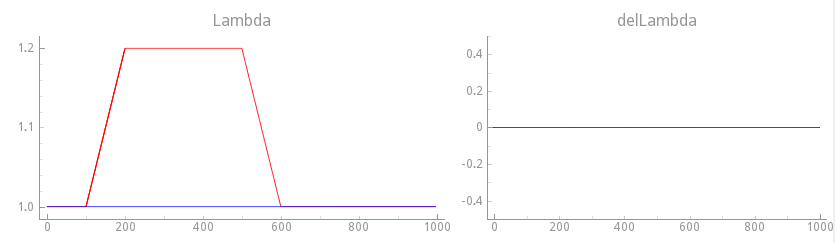
Experiment exp16 - stretch resting myocyte, velocity dependence off
To observe the effect of cellular stretch upon EP we apply now mechanical loading protocols
to the resting myocyte.
As a reference case, we apply a step change in stretch of 20%
and observe only length-dependent effects, that is, velocity-dependence is turned off.
This is achieved with the loading protocol shown in fig-gpb-land-mef-ld-protocol.
./run.py --experiment passive --EP augustin --duration 2000 --bcl 1000 \
         --ID exp16 --init exp15/exp15_augustin_bcl_1000_ms_dur_2000_ms.sv \
         --fs traces/lambda_step_tr_time_100ms.dat --overlay exp15 \
         --visualize --vis_var V Cai Tension Lambda delLambda
Expected result: Now mechanics feed back to EP: stretch alters Ca transient and AP.
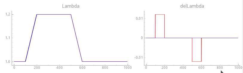
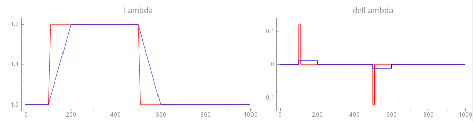
Experiment exp17 - stretch resting myocyte, velocity dependence on, slower transition
We repeat experiment exp16 now, but with velocity dependence enabled.
First, we use a moderately fast step change by going from \(\lambda=1.0\)
to \(\lambda=1.2\) in 100 ms and compare results with exp16
where velocity dependence was disabled. See fig-gpb-land-mef-ld-vd-slow-protocol.
./run.py --experiment passive --EP augustin --duration 2000 --bcl 1000 \
         --ID exp17 --init exp15/exp15_augustin_bcl_1000_ms_dur_2000_ms.sv \
         --fs traces/lambda_step_tr_time_100ms.dat --fsDot traces/dlambda_step_tr_time_100ms.dat \
         --overlay exp16 --visualize --vis_var V Cai Tension Lambda delLambda
Experiment exp18 - stretch resting myocyte, velocity dependence on, faster transition
We repeat experiment exp16 now, but with velocity dependence enabled.
We use a faster step change by going from \(\lambda=1.0\)
to \(\lambda=1.2\) in only 10 msecs. See fig-gpb-land-mef-ld-vd-fast-protocol.
./run.py --experiment passive --EP augustin --duration 1000 --bcl 1000 \
         --ID exp18 --init exp15/exp15_augustin_bcl_1000_ms_dur_2000_ms.sv \
         --fs traces/lambda_step_tr_time_10ms.dat --fsDot traces/dlambda_step_tr_time_10ms.dat \
         --overlay exp17 --visualize --vis_var V Cai Tension Lambda delLambda
Strongly coupled electro-mechanical human ventricular myocyte model with passive component
In this set last set of experiments we couple the recent EP model of the human ventricular myocyte due to Tomek et al 2020 11 (Tomek20) with the active tension model due to Land et al 2017 12 (Land17) with dynamic sarcomere length capabilities (_DynSarc) Details on the implementation and parameterization of the coupling have been reported in Margara et al 13 .
Experiment exp19 - pace to limit cycle
We pace the model for 20 seconds to arrive at a limit cycle.
./run.py --EP tomek20land17_dynsarc --duration 20000 \
         --bcl 1000 --ID exp19 --visualize --vis_var V Cai stretch delLambda Tension
Expected result: Action potential traces, Ca and tension transients converge to a limit cycle. We see a time varying stretch of the sarcomere.
Experiment exp20 - confirm limit cycle
Using the state of the myocyte stored in the file
exp19_tomek20land17_dynsarc_bcl_1000_ms_dur_20000_ms.sv in exp19,
we confirm now that your trajectories are close to a limit cycle for the
given bcl and stretch we run
./run.py --EP tomek20land17_dynsarc --duration 2000 \
         --bcl 1000 --ID exp20 \
         --init exp19/exp19_tomek20land17_dynsarc_bcl_1000_ms_dur_20000_ms.sv \
         --visualize --vis_var V Cai stretch delLambda Tension
Expected result: You should see stable action potential traces, Ca transients, and a periodic tension transient with little variation from the first to the second beat.
Experiment exp21 - return to rest
Again, as this model is strongly coupled, mechanical loading influences EP in the myocyte. To observe MEF effects we leave the limit cycle and stop pacing for 2 seconds. That is, in this experiment we keep the myocyte quiescent, we do not deliver an electrical stimulus current, nor a mechanical stretch protocol and observe the return of trajectories to a resting state.
./run.py --experiment passive --EP tomek20land17_dynsarc \
         --duration 4000 --bcl 1000 --ID exp21 \
         --init exp19/exp19_tomek20land17_dynsarc_bcl_1000_ms_dur_20000_ms.sv \
         --visualize --vis_var V Cai stretch delLambda Tension
Expected result: With no pacing or stretch, voltage, calcium, and tension all relax back to rest. Strong coupling ensures electrical and mechanical variables return to equilibrium together.
Using your own models
In addition to the built-in models, you can integrate your own EP and stress models into the simulation framework. This allows you to test new hypotheses, validate custom ionic formulations, or explore novel myofilament dynamics.
Experiment exp22 - own EP model + Land17 stress
Use your own EP .model file or download an electrophysiology model from CellML
(see Converting CellML example).
Exemplatory we use a version of the tenTusscherPanfilov model located in models
(models/own_tenTusscherPanfilov.model)
./run.py --load-module models/own_tenTusscherPanfilov.model --stress stress_land17 \
         --duration 20000 --bcl 500 --ID exp22 \
         --visualize --vis_var V Cai Tension
Expected result:
The python script automatically compiles the ionic model using make_dynamic_model.sh.
The following bench simulation produces similar AP, Ca, and tension transient as above.
Experiment exp23 - own strongly coupled model
Finally, you can define a fully coupled electromechanical model where your
EP and stress formulations interact via mechano-electric feedback (MEF)
(models/own_tenTusscherPanfilovLand17.model).
./run.py --load-module models/own_tenTusscherPanfilovLand17.model \
         --duration 20000 --bcl 500 --ID exp23 \
         --visualize --vis_var V Cai Tension
Expected result:
The python script automatically compiles the ionic model using make_dynamic_model.sh.
The following bench simulation produces similar AP, Ca, and tension transient as above.
References
Niederer SA, Plank G, Chinchapatnam P, Ginks M, Lamata P, Rhode KS, Rinaldi CA, Razavi R, Smith NP. Length-dependent tension in the failing heart and the efficacy of cardiac resynchronization therapy, Cardiovasc. Res. 89(2):336-43, 2011. DOI: 10.1093/cvr/cvq318↩︎
Crozier A, Blazevic B, Lamata P, Plank G, Ginks M, Duckett S, Sohal M, Shetty A, Rinaldi CA, Razavi R, Smith NP, Niederer SA. The relative role of patient physiology and device optimisation in cardiac resynchronisation therapy: A computational modelling study, J. Mol. Cell Cardiol. 96:93-100, 2026 DOI: 10.1016/j.yjmcc.2015.10.026↩︎
Land S, Niederer SA, Aronsen JM, Espe EK, Zhang L, Louch WE, Sjaastad I, Sejersted OM, Smith NP An analysis of deformation-dependent electromechanical coupling in the mouse heart, J. Physiol. 590(18):4553-69, 2012. DOI: 10.1113/jphysiol.2012.231928↩︎
Land S, Park-Holohan SJ, Smith NP, Dos Remedios CG, Kentish JC, Niederer SA. A model of cardiac contraction based on novel measurements of tension development in human cardiomyocytes, J. Mol. Cell Cardiol. 106:68-83, 2017. DOI: 10.1016/j.yjmcc.2017.03.008↩︎
Augustin CM, Neic A, Liebmann M, Prassl AJ, Niederer SA, Haase G, Plank G. Anatomically accurate high resolution modeling of human whole heart electromechanics: A strongly scalable algebraic multigrid solver method for nonlinear deformation, J. Comput. Phys. 305:622-646, 2016. DOI: 10.1016/j.jcp.2015.10.045↩︎
Grandi E, Pasqualini FS, Bers DM. A novel computational model of the human ventricular action potential and Ca transient, J. Mol. Cell Cardiol. 48, 112-121, 2010. DOI: 10.1161/CIRCRESAHA.111.253955↩︎
Land S, Niederer SA, Aronsen JM, Espe EK, Zhang L, Louch WE, Sjaastad I, Sejersted OM, Smith NP An analysis of deformation-dependent electromechanical coupling in the mouse heart, J. Physiol. 590(18):4553-69, 2012. DOI: 10.1113/jphysiol.2012.231928↩︎
Tondel K, Land S, Niederer SA, Smith NP. Quantifying inter-species differences in contractile function through biophysical modelling, J. Physiol. 593(5):1083-111, 2015. DOI: 10.1113/jphysiol.2014.279232↩︎
Tomek J, Bueno-Orovio A, Rodriguez B. ToR-ORd-dynCl: an update of the ToR-ORd model of human ventricular cardiomyocyte with dynamic intracellular chloride, bioRxiv, 2020. DOI: 10.1101/2020.06.01.127043↩︎
Land S, Park-Holohan SJ, Smith NP, Dos Remedios CG, Kentish JC, Niederer SA. A model of cardiac contraction based on novel measurements of tension development in human cardiomyocytes, J. Mol. Cell Cardiol. 106:68-83, 2017. DOI: 10.1016/j.yjmcc.2017.03.008↩︎
Margara F, Wang ZJ, Levrero-Florencio F, Santiago A, Vasquez M, Bueno-Orovio A, Rodriguez B. In-silico human electro-mechanical ventricular modelling and simulation for drug-induced pro-arrhythmia and inotropic risk assessment, Prog. Biophys. Mol. Biol. 159:58-74, 2021. DOI: 10.1016/j.pbiomolbio.2020.06.007↩︎
Recent questions tagged examples, experiments, parameters, land
There are tagged with examples, experiments, parameters, land.
Here we display the 5 most recent questions. You can click on each tag to show all questions for this tag.
You can also ask a new question.