Stimulation

See code in GitLab.
Author: Gernot Plank gernot.plank@medunigraz.at and Moritz Linder moritz.linder@kit.edu

cd ${TUTORIALS}/02_EP_tissue/02_stimulation 

Electrical Stimulation

Basically, cardiac tissue can be stimulated either by changing the electrical potential or by injection/withdrawal of currents. In both cases stimulation can be applied in the intracellular domain, \(\Omega_{\rm i}\), or in the extracellular domain, \(\Omega_{\rm e}\). Mathematically, voltage stimuli correspond to Dirichlet boundary conditions whereas current stimuli are implemented either as Neumann boundary condition or, alternatively, as volume sources. The choice of stimulation procedure should be based on the experimental conditions to be modelled and the electronic circuitry used in the voltage/current source. If stimulation is mediated via controlled injection of currents the current stimulation methods is preferible, otherwise if voltage sources are used the voltage stimulation method should be used. A special case is the stimulation with a transmembrane current where current is injected in one domain and withdrawn in the other domain at the exact same location. Thus the stimulus itself does not set up a primary extracellular field as there is no current path between injecting and withdrawing electrode.

Extracellular Voltage Stimulation

Mathematically, intracellular voltage stimulation is easily feasible, but since this is of very limited practical relevance support for this type of stimulation is not implemented. Voltage stimulation is therefore always applied in the extracellular domain \(\Omega_{\rm e}\). This is achieved by applying Dirichlet boundary conditions in \(\Omega_{\rm e}\) which directly alter extracellular potentials. If we consider the bidomain equation governing the extracellular potential field

\[\nabla \cdot \sigma_{\rm e} \nabla \phi_{\rm e} = -\beta I_{\rm m}\]

or in the elliptic-parabolic cast given by

\[\nabla \cdot (\sigma_{\rm e} + \sigma_{\rm e} \nabla \phi_{\rm e}) = 0\]

extracellular voltage stimulatin is achieved by enforcing the extracellular potential \(\phi_{\rm e}^{\rm p}(t)\) to follow a given time course, i.e. the prescribed stimulus pulse shape, over the entire electrode surface, \(\Gamma_{\rm D}\)

\[\phi_{\rm e} = f(t) \hspace{0.5cm} \forall x \in \Gamma_{\rm D}\]

or, alternatively, also a spatial variation of extracellular potentials :math:`phi{rm e}(x)' is possible, that is,

\[\phi_{\rm e} = f(t,x) \hspace{0.5cm} \forall x \in \Gamma_{\rm D} .\]

In practice, voltage stimulation is performed with voltage sources. Voltage sources have two terminals which impose a potential relative to a reference usually referred to as ground (GND). Often one terminal is grounded, i.e. connected to a zero potential, whereas the other terminal prescribes the time course of the chosen pulse shape. Many other variations are also possible, but not all will be discussed. In the following we restrict ourselves to configurations which are realized typically in stimulation circuits.

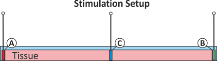
For testing the various types of extracellular stimulation we generate a thin strand of tissue of 1 cm length. Electrodes are located at both caps of the strand with an additional auxiliary electrode in the very center of the strand. An illustration of the setup is given in fig-extra-stim-setup. Extracellular voltage and current stimuli are pre-configured to generate an extracellular voltage drop across the strand of about 2 V. This corresponds to an electric field magnitude of 2 V/cm which is sufficient to initiate action potential propagation under the cathode.

Experiments

Several types of stimulation setups are predefined. Run

./run.py --help 

to see all exposed experimental parameters. The input parameter stimulus selects a stimulus configuration among the following available options:

--stimulus {extra_V, extra_V_bal, extra_V_OL, extra_I, extra_I_bal, extra_I_mono}  # pick stimulus type
--grounded {on, off}  # turn on/off use of ground wherever possible

The geometry of the three electrodes A, B and C are defined as follows:

# electrode A
stim[0].elec.p0[0] = -5050.
stim[0].elec.p1[0] = -4950. 
stim[0].elec.p0[1] = -100.
stim[0].elec.p1[1] = 100.
stim[0].elec.p0[2] = -100. 
stim[0].elec.p1[2] = 100. 

# electrode B
stim[1].elec.p0[0] = 4950.
stim[1].elec.p1[0] = 5050.
stim[1].elec.p0[1] = -100.
stim[1].elec.p1[1] = 100.
stim[1].elec.p0[2] = -100.
stim[1].elec.p1[2] = 100.

# electrode C
stim[2].elec.p0[0] = -10.
stim[2].elec.p1[0] = 10.
stim[2].elec.p0[1] = -5000.
stim[2].elec.p1[1] = 5000.
stim[2].elec.p0[2] = -5000.
stim[2].elec.p1[2] = 5000.

Experiment exp01 (Extracellular Voltage Stimulation with Ground)

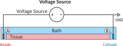
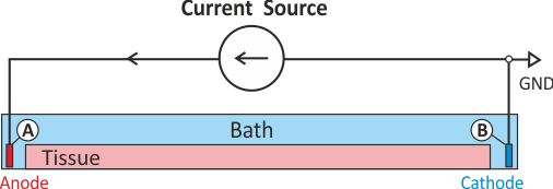
This is the default setup for modeling extracellular voltage stimulation where one terminal of the voltage sources is used to prescribe the time course of the extracellular potential \(\phi_{\rm e}\) at one electrode, and enforce a zero potential at the corresponding electrode. If the enforced potentials are positive, that is \(\phi_{\rm e}^{\rm p} > 0\) holds, the positive terminal acts as an anode and the grounded terminal acts as a cathode. Such a configuration sets up an electric stimulation circuit as shown in fig-extraV-wgnd. On theoretical grounds, there is no necessity for using a ground electrode in this case as a unique solution for the elliptic problem can be found by using one Dirichlet boundary conditions, that is, using the electrode prescribing the stimulus pulse would suffice. However, such a setup cannot be realized with an electric circuit and as such it is unlikely to be suitable for matching a given experimental scenario.

The stimulus option extra_V sets up stimulation through application of extracellular voltage corresponding to fig-extraV-wgnd. The potential electrode A is clamped to 2000 mV for a duration of 2 ms, electrode B is grounded, i.e., \(\phi_{\rm e} = 0\).

Electrode C is not used here, electrodes A and B are configured as follows:

numstim = 2                      # use two electrodes, A and B

# electrode A
stim[0].crct.type = 2            # extracellular voltage stimulus
stim[0].pulse.strength = 2e3     # voltage at A in mV 

# electrode B
stim[1].crct.type = 3            # extracellular ground

Run this experiment by executing

./run.py --stimulus extra_V --visualize

Experiment exp02 (Balanced Extracellular Voltage Stimulation)

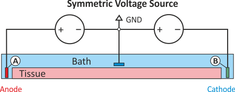
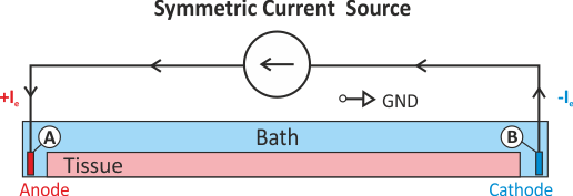
The extracellular potential distribution \(\phi_{\rm e}^{\rm p}(\rm{x})\) induced by the standard setup for extracellular voltage stimulation is not symmetric. Under various circumstances it may be convenient to enforce an extracellular electric field which is symmetric with regard to the two electrodes. Such a potential distribution can be enforced using two electrodes of exactly opposite polarity and an additional ground which then the zero potential isoline to run through the location of the grounding electrode. This setup is shown in fig-extraV-symm-wgnd.

As in experiment exp01, the stimulus option extra_V_bal sets up stimulation through the application of extracellular voltage. The potential on the left cap is clamped to 1000 mV for a duration of 2 ms and the right hand electrode to -1000mV. This stimulation circuit corresponds to the setup shown in fig-extraV-symm-wgnd.

numstim = 3                      # use all three electrodes, A, B and C

# electrode A
stim[0].crct.type =  2           # extracellular voltage stimulus
stim[0].pulse.strength =  1e3    # voltage at A in mV 

# electrode B
stim[1].crct.type =  2           # extracellular voltage stimulus
stim[1].pulse.strength = -1e3    # voltage at B in mV

# electrode C
stim[2].crct.type =  3           # extracellular ground at C

Realize this experiment by running

./run.py --stimulus extra_V_bal --visualize

Experiment exp03 (Extracellular Voltage Stimulation with Circuit Break)

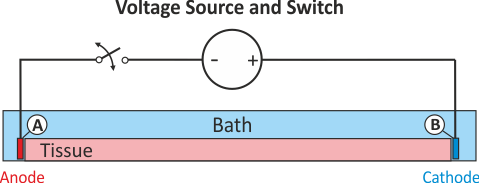
Depending on a given hardware, a switch may or may not interrupt the circuit after pulse delivery. If a switch remains closed for the entire simulation the potential at both electrodes are governed by the potentials of the terminals of the voltage source. Typically, the potential at both terminals will be zero after the pulse delivery, that is, both electrodes act as GND. This may not always be desired. If a switch interrupts the circuit after delivery the potential at one terminal is allowed to float whereas the other terminal will act as ground. An illustration of the difference between the two modes is given in fig-extraV-wgnd-switched.

As in experiment exp01, the stimulus option extra_V_OL sets up stimulation through the application of extracellular voltage. The extracellular potential at electrode A is clamped to 2000 mV for a duration of 2 ms. In contrast to the extra_V electrode A is disconnected from the source after stimulus delivery. Therefore, the potential at A is allowed to float after the end of the stimulus, that is, electrode A won't act as a ground after delivery of the voltage pulse. This stimulation circuit corresponds to the setup shown in fig-extraV-wgnd-switched.

numstim = 2                      # use two electrodes, A and B

# electrode A
stim[0].crct.type = 5            # extracellular voltage stimulus, switched
stim[0].pulse.strength = 2e3     # voltage at A in mV 

# electrode B
stim[1].crct.type = 3            # extracellular ground

To realize this scenario, run

./run.py --stimulus extra_V_OL --visualize

Extracellular Current Stimulation

In many cases tissue is stimulated by injecting current through a current source. Modelingwise current stimulation is simpler to implement as there is no need for manipulating the left hand side of the equation system. Mathematically, current injection is modelled either as a Neumann boundary condition given as

\[\sigma_{\rm e} \nabla \phi_{\rm e} \cdot n = I_{\rm en} \hspace{5mm} \text{at} \hspace{5mm} \Gamma_{\rm en}\]

or, alternatively, as a volmetric current source given as

\[\nabla \cdot \sigma_{\rm e} \nabla \phi_{\rm e} = -I_{\rm e}\]

where \(I_{\mathbf e}\) is the volumetric current density. While there are FEM-theoretical advantages of using a Neumann approach, in terms of ease of implementation volumetric sources are more flexible and easier to handle. A Neumann approach injects current through the surface of an electrode into the surrounding domain. This is straight forward to implement when electrodes are located at the boundary of the extracellular domain \(\Omega_{\rm e}\). However, in many scenarios this is not the case, for instance, when modeling current injection into the blood pool of the right ventricle (RV) using a RV coil electrode of an implanted device. In this case elements enclosed by the surface of the Neumann electrode should be removed. The use of volumetric sources is simpler in this regard. Electrodes can be located at arbitrary locations. The downside of volumetric sources is that this method is not entirely mesh independent (current is injected via the FEM hat functions and the total volume therefore varies due to variability in the surface representation). openCARP implements volumetric sources, Neumann current sources are not implemented. In those cases where mesh resolution dependence is unacceptable the total current to be injected can be prescribed which is used for internal scaling of current density such that the prescribed total current is injected indepdently of mesh resolution.

It should be noted that the elliptic PDE as given in Eq. extra_stim_V2 which has to be solved to find the extracellular potential distribution \(\phi_{\rm e}(x)\) is a pure Neumann problem and as such is singular. That is, the solution can only be determined up to a given constant as the Nullspace of a scalar Neumann problem comprises all constant functions. Without using a Dirichlet boundary condition the problem cannot be solved therefore unless an additional equation is used to constrain the solution in a unique way. An often used constraint is to enforce the average potential in the domain to be zero, that is

\[\int_{\Omega_{\rm e}} \phi_{\rm e}(x) d\Omega = 0 .\]

Such constraints can be imposed with various stabilization techniques.

Experiment exp04 (Extracellular Current Stimulation with Ground)

The standard setup for extracellular current stimulation comprises an electrode for current injection combined with a ground electrode. The ground electrode enforces a homogeneous Dirichlet boundary thus rendering the problem non-singular and solvable without any additional constraints. Assuming the current source delivers a positive current pulse current is being injected in electrode A thus lifting the extracellular potential \(\phi_{\rm e}\) there (fig-extraI-wGND). The increase in \(\phi_{\rm e}\) drives the transmembrane voltage \(V_{\rm m}\) towards more negative values, thus electrode A hyperpolarizes tissue in its adjacency and acts therefore as an anodal stimulus. Electrode B is grounded. Any current injected in A is automatically collected electrode B without the need of explicitly withdrawing current there. As current is withdrawn at electrode B, \(\phi_{\rm e}\) is being lowered there which drives \(V_{\rm m}\) towards more positive values. Thus electrode B depolarizes tissue in its adjacency and acts therefore as a cathodal stimulus.

The stimulus option extra_I sets up stimulation through the application of an extracellular current. The current is injected into electrode A in the extracellular medium and withdrawn at electrode B which, in turn, is grounded. The extracellular current strength is chosen to induce an extracellular potential drop of 2000 mV across the strand as before with extracellular voltage stimulation in extra_V. This configuration corresponds to the setup shown in fig-extraI-wGND. Electrode C is not used here, while electrodes A and B are configured as follows:

numstim = 2                      # use two electrodes, A and B

# electrode A
stim[0].crct.type = 1            # extracellular current stimulus
stim[0].pulse.strength = 3.1e6   # current density at A in µA/cm^3

# electrode B
stim[1].crct.type = 3            # extracellular ground

To see the result, run

./run.py --stimulus extra_I --visualize

Experiment exp05 (Balanced Extracellular Current Stimulation)

Similar to the scenario described above, the standard setup for extracellular current stimulation does not generate a symmetric potential field. However, a symmetric potential field can be setup by using two current electrodes, for instance, electrode A is used for injection and electrode B for withdrawing currents. However, in this case an additional difficulty arises stemming from the fact that we attempt to solve a pure Neumann problem. There are a two things to keep in mind:

When solving a pure Neumann problem one has to comply with the compatibility condition which boils down to the fact that the sum of all currents injected and withdrawn must balance out to zero. If we integrate over Equations we obtain

\[\int_{\Omega} \nabla \cdot \sigma_{\rm e} \nabla \phi_{\rm e} \, d\Omega = -\int_{\Omega} I_{\rm e} \, d\Omega \ \sigma_{\rm e} \nabla \phi_{\rm e} \cdot n = \int_{\Omega} I_{\rm en} \nonumber\]

Using Gauss' diverence theorem we obtain the compatibility condition

\[\int_{\Omega} \nabla \cdot \sigma_{\rm e} \nabla \phi_{\rm e} \, d\Omega = \int_{\Gamma} \sigma_{\rm e} \nabla \phi_{\rm e} \cdot n \, d\Gamma - \int_{\Omega} I_{\rm e} \, d\Omega\]

essentially meaning that all extracellular stimulus currents must add up to zero.

A pure Neumann problemcan be solved without a Dirichlet condition by resorting to solver techniques which deal with the nullspace of the problem. Typically, a condition such as Eq. extra_stim_I3 is enforced. This can be considered to be a diffuse floating ground (see fig-extraI-symm-diffuse)`

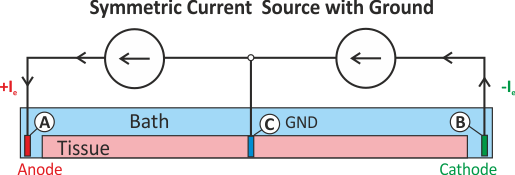
A setup with two current electrodes can be augmented with an additional reference electrode. In this case the compatibility condition does not need to be enforced. However, failure to balance the currents turns the ground electrode into an anode or cathode as any excess current will be collected by the ground electrode. Such a setup is shown in fig-extraI-symm-wgnd.

Similar to experiment exp04, the stimulus option extra_I_bal sets up stimulation through the injection of extracellular current with the difference being that B is not grounded. Extracellular current is injected into electrode A and the same amount is withdrawn from electrode B. Both configurations also induce an extracellular potential drop of 2000 mV across the strand, albeit in a symmetric way. Note that in both cases, the compatibility condition must be satisfied. This is taken care of by openCARP internally by balancing the total current injected/withdrawn through electrodes A and B. If balancing is imperfect, a stimulation would also occur around electrode C as all the excess current would drain there.

In the setup with an explicit ground, electrodes are defined as:

numstim = 3                         # use all three electrodes, A, B and C

# electrode A
stim[0].crct.type =  1              # extracellular voltage stimulus
stim[0].pulse.strength =  3.1e6     # current density at A in µA/cm^3 

# electrode B
stim[1].crct.type =  1              # extracellular voltage stimulus
stim[1].crct.balance  =  0          # no strength prescribed, balance with stimulus[0]

# electrode C
stim[2].crct.type =  3              # extracellular ground at C

To solve the pure Neumann problem without an explicit ground, the input parameter grounded is set to on. In fact, openCARP turns on this mode automatically if a pure Neumann configuration is detected.

numstim = 2                         # use electrodes A and B 

# electrode A
stim[0].crct.type =  1              # extracellular voltage stimulus
stim[0].pulse.strength =  3.1e6     # current density at A in µA/cm^3 

# electrode B
stim[1].crct.type =  1              # extracellular voltage stimulus
stim[1].crct.balance  =  0          # no strength prescribed, balance with stimulus[0]

In order to finally execute the last experiment, run

./run.py --stimulus extra_I_bal --visualize

Recent questions tagged experiments, examples, stimulus, tissue