N-version benchmark of cardiac tissue electrophysiology

See code in GitLab.
Author: Moritz Linder moritz.linder@kit.edu, Tobias Gerach tobias.gerach@kit.edu

Overview

cd ${TUTORIALS}/02_EP_tissue/03E_study_resolution

This example implements the classic benchmark problem for electrophysiology introduced by Niederer et al. in 2011. [Niederer2011]

Problem definition

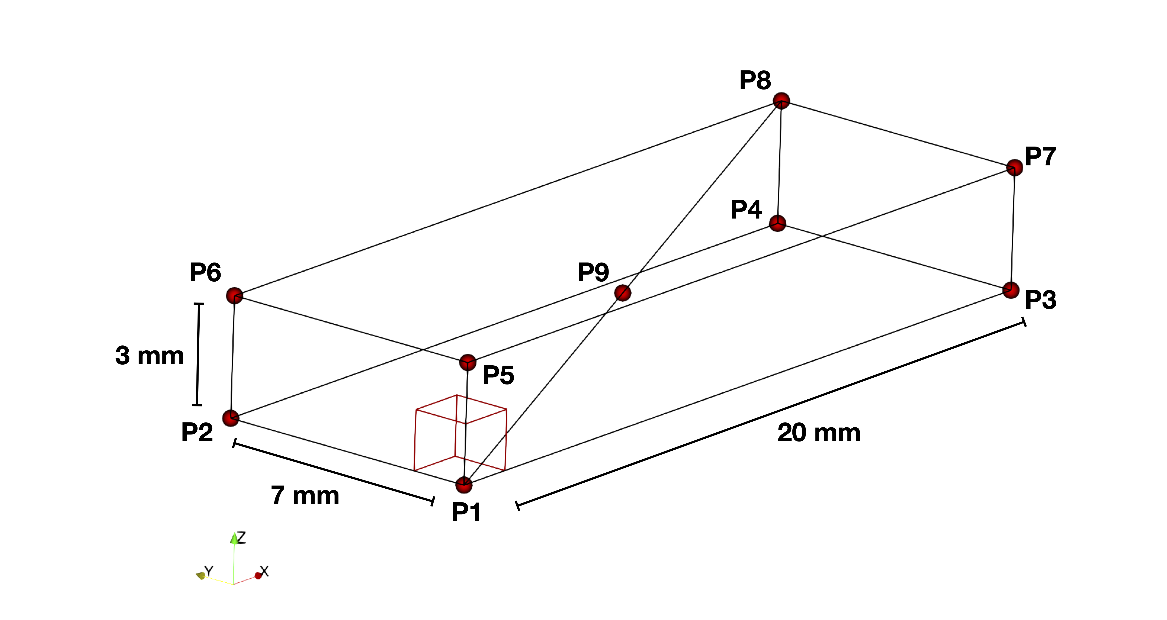
The geometry of the tissue model is defined by a cuboid with dimensions 20.0 x 7.0 x 3.0 mm. Fiber directions are defined to be oriented in the X axis of the cuboid. All boundaries are assumed to have a zero-flux boundary condition. The stimulus current is delivered to a volume of 1.5 x 1.5 x 1.5 mm originating at the corner of the slab with coordinates \(x=y=z=0\).

The ionic model that is used in the benchmark is the ten Tusscher & Panfilov model [TTP] with the epicardial cell model variant. This is set in the base parameter file alongside a single cell surface-to-volume ratio of \(0.14 \mu m^{-1}\) and the portion of the volume that is occupied by cells (=1). To use a given set of initial values for the state variables, we load the state variable file singlecell.sv with the parameter -imp_region[0].im_sv_init.

num_imp_regions = 1 
imp_region[0].name = "Ventricle" 
imp_region[0].im   = tenTusscherPanfilov
imp_region[0].im_param = "flags=EPI"
imp_region[0].cellSurfVolRatio = 0.14
imp_region[0].volFrac = 1

The tissue is assumed to be transverse isotropic. Therefore, we set a single conductivity region with the intra- and extracellular conductivites in longitudinal and transversal directions.

num_gregions    = 1
gregion[0].g_il = 0.17
gregion[0].g_it = 0.019
gregion[0].g_in = 0.019
gregion[0].g_el = 0.62
gregion[0].g_et = 0.24
gregion[0].g_en = 0.24

To set up the stimulus current, we define a box by providing the lower left corner \(p0 = (0,0,0)\) and the upper right corner \(p1 = (1500,1500,1500)\). The stimulation protocol is set to start at 0 s with a duration of 2 ms and a pulse strength of \(50000 \mu A cm^{-3}\).

num_stim                = 1
stim[0].elec.geom_type  = 2
stim[0].elec.p0[0]      = 0
stim[0].elec.p0[1]      = 0
stim[0].elec.p0[2]      = 0
stim[0].elec.p1[0]      = 1500
stim[0].elec.p1[1]      = 1500
stim[0].elec.p1[2]      = 1500
stim[0].pulse.strength  = 35.71
stim[0].ptcl.duration   = 2.00
stim[0].ptcl.start      = 0.00

A quantitative comparison of the benchmark simulations is achieved by comparing activation times at certain points of the geometry and along a diagonal line from one corner of the cuboid to another. An activation time is recorded at the time the membrane potential passes through 0 mV for the first time. This is achieved by setting the following parameters:

num_LATs             =         1
lats[0].measurand    =         0 
lats[0].all          =         0
lats[0].mode         =         0
lats[0].threshold    =         0.
lats[0].method       =         1

Usage

The experiment specific options are:

--tend
            duration of the simulation in ms

--dx
            resolution of the mesh in um to be used for benchmark

--dt
            temporal resolution in us

--massLumping
            toggle mass massLumping on (1) or use full mass matrix (0)

--plot
            generate a plot of activation times along the block diagonal

--compare
            run benchmark with --dx 100 200 and 500 and make comparison plot

The user can either run single experiments by calling python3 run.py with the optional arguments --tend, --dx, --dt, and --massLumping or run the entire benchmark setup with the argument --compare.

--compare

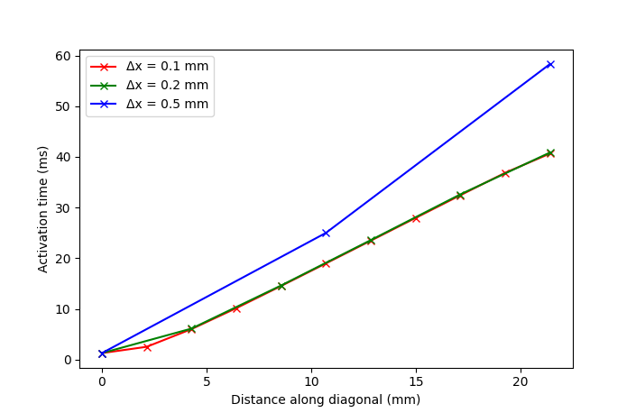
With this option you will run all simulations required for the benchmark and create a comparison plot for the activation times on the block diagonal with \(\Delta x = 0.5, 0.2, 0.1\) mm resolution.

Notice that the accuracy of the solution deteriorates with lower resolution meshes.

--compare with mass lumping

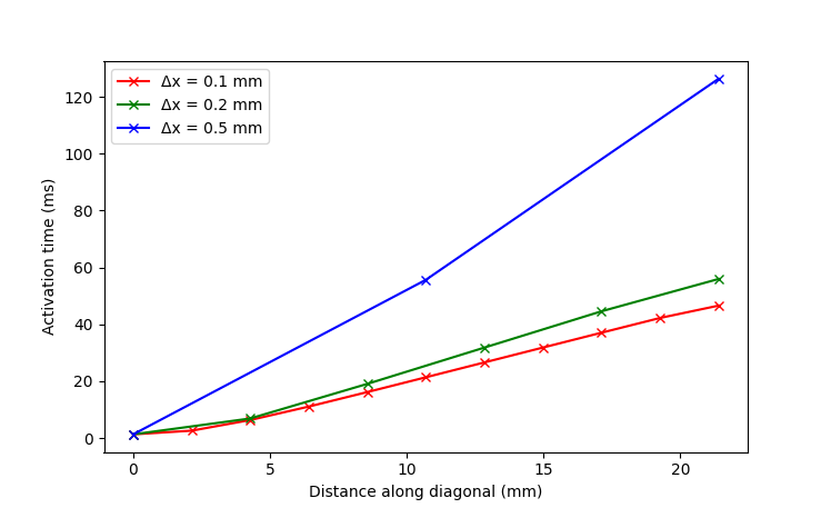
Now we will run the benchmark setting with the additional parameter --massLumping 1 to see how mass lumping affects the solution in the otherwise unchanged setup.

Mass lumping is a common numerical technique in FEM to speed up computation. However, notice how the accuracy of the solution deteriorates even faster than before. This was one of the beneficial outcomes of the benchmark, which showed that mass lumping was leading to the biggest inaccuracies among finite element codes especially with lower spatial resolutions. Therefore, you should always remember to consider the tradeoffs of this numerical technique.

References