Effective Refractory Period (ERP) Restitution

See code in GitLab.
Author: Patricia Martinez patricia.martinez@ihu-liryc.fr

Introduction

Refractoriness is an electrophysiological property that characterizes the response of cardiac tissue to premature stimulation. Shortened cardiac refractoriness has shown to promote sustained re-entrant activity and can be assessed during electrophysiological studies following the extra-stimulus S1S2 pacing technique, in which a train of S1 stimuli is given at a certain cycle length followed by a premature S2 stimulus. The effective refractory period (ERP) can then be defined as the longest S1S2 interval that fails to elicit a response (i.e.,capture) in the tissue ¹ . An S1S2 protocol is illustrated in fig-S1S2-protocol

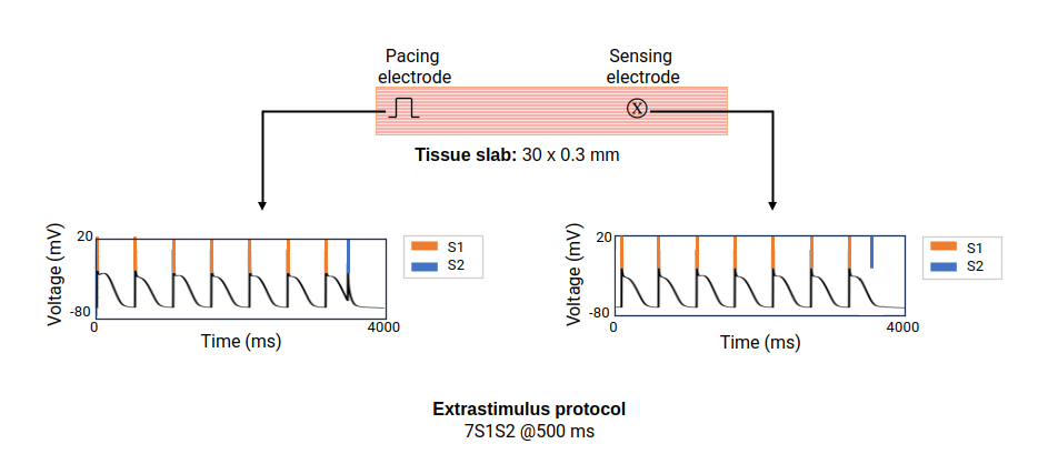
Figure 1. S1S2 pacing protocol: The tissue slab is paced with a train of seven S1 stimuli at 500 ms, followed by a premature stimulus S2 that is progressively shortened until it fails to activate the tissue near the sensing electrode.

In this experiment we are using the Courtemanche et al. mathematical model ² to simulate single-cell atrial electrophysiology. We also modify the maximum ionic conductances of key ionic channels affecting the action potential morphology to reflect electrical remodeling due to atrial fibrillation (AF) ³ . You can observe the differences in the action potential morphology in the following figure:

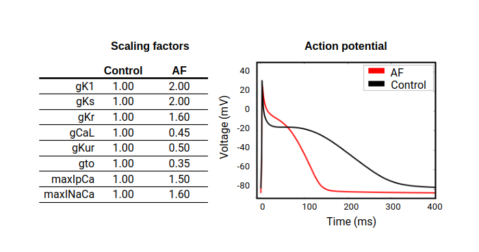
Figure 2. Changes to the action potential due to electrical remodeling: the action potential of a normal atrial myocyte (control) is shown in black and the changes due to electrical remodeling in atrial fibrillation (AF) are shown in red. The table includes the scaling factors applied to each ionic conductance.

ERP Detection Algorithm (Bisection Method)

The bisection method is used to efficiently determine the ERP based on a given set of input parameters ⁴ . The algorithm iteratively narrows the S1S2 interval until the ERP is estimated within a defined tolerance, as described below.

Input:
    S1         ← basic cycle length
    s2_min     ← minimum initial S1–S2 interval
    s2_max     ← maximum initial S1–S2 interval
    tolerance  ← desired precision (e.g., 1 ms)
    APD        ← action potential duration (initial estimate for ERP search)
    ACT        ← time window for activation detection

Output:
    ERP        ← effective refractory period
    DI         ← diastolic interval
    APD        ← action potential duration

Initialize:
    start_S1 ← fixed start time of S1 stimuli (defined by prepace time)
    last_active_s2 ← None

while (s2_max - s2_min) > tolerance do:
    s2 ← (s2_min + s2_max) / 2

    start_S2 ← start_S1 + s2
    tsav_state ← start_S2 + ACT + APD + margin

    Run simulation with both stimuli s1 and s2

    if activation is detected after S2:
        last_active_s2 ← s2
        s2_min ← s2
    else:
        s2_max ← s2

ERP ← last_active_s2
DI  ← S1 - APD

return ERP, DI, APD

ERP Restitution

Restitution describes how the cardiac tissue adapts to changes in pacing rate. In general, restitution refers to the relationship between the action potential duration, conduction velocity or refractory period and the preceding diastolic interval (DI) or cycle length. ERP restitution describes how the effective refractory period changes as a function of the preceding basic cycle length (S1 interval).

Usage

To run the tutorial, change directories as follows:

cd ${TUTORIALS}/02_EP_tissue/03F_ERP_restitution

The following input parameters are available:

python3 run.py --help

--model               Ionic model name from LIMPET library (default: Courtemanche)

--S1                  Pacing cycle length (ms) of S1 stimulus (default: 500 ms)

--cv                  Conduction velocity (m/s) (default: 0.7 m/s)

--model_par           Scaling factors of ionic channel conductances (leave empty for normal action potential morphology)

--restitution         Flag to enable ERP restitution protocol and plot curve. Optionally set the minimum S1 value (default: 200 ms)

Preparation for S1S2 Protocol

To reach a steady state, single cells are paced 100 times (--numstim) at a fixed basic cycle length of 500 ms (--cell_bcl).Then the entire tissue slab is stimulated 7 times (--prebeats), and the action potential duration at 94% (--APD_percent) of the final beat is measured. This APD is then used as an initial estimate for ERP calculation. Additionally, if no conductivities are provided (--giL, --geL), monodomain tissue conductivities for a given conduction velocity (--cv) are calculated by calling tuneCV inside the experiment.

tuneCV --velocity 0.7 --resolution 300 --model Courtemanche --modelpar "GK1*2,GKs*2,GKr*1,GCaL*0.45,factorGKur*0.5,Gto*0.35,maxIpCa*1.5,maxINaCa*1.6" --dt 20 --tol 0.001 --lumping True --sourceModel monodomain --surf True --converge True

To run this experiment, type the following in the terminal:

python3 run.py  --model Courtemanche --S1 500 --cv 0.7 --model_par "GK1*2,GKs*2,GKr*1,GCaL*0.45,factorGKur*0.5,Gto*0.35,maxIpCa*1.5,maxINaCa*1.6"

To calculate ERP restitution by varying the pacing cycle length of the S1 stimulus, add the --restitution flag to use default parameters:

python3 run.py  --model Courtemanche --S1 500 --restitution --cv 0.7 --giL 0.40500 --geL 1.45474 --model_par "GK1*2,GKs*2,GKr*1,GCaL*0.45,factorGKur*0.5,Gto*0.35,maxIpCa*1.5,maxINaCa*1.6"

You can also modify the pacing protocol. For example, in this case, the initial S1 is set to 600 ms and will decrease to 100 ms in steps of 50 ms:

python3 run.py  --model Courtemanche --S1 600 --restitution 100 --S1_step 50 --cv 0.7  --giL 0.40500 --geL 1.45474 --model_par "GK1*2,GKs*2,GKr*1,GCaL*0.45,factorGKur*0.5,Gto*0.35,maxIpCa*1.5,maxINaCa*1.6"

The previous command generates the restitution curve shown in fig-erp_restitution

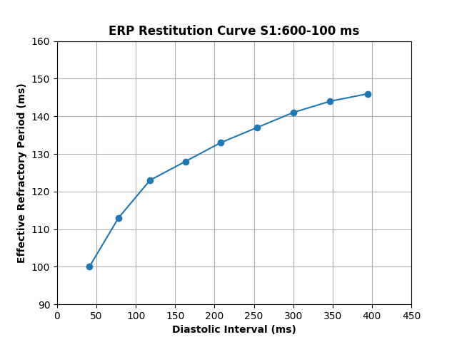
Figure 3. Effective refractory period restitution curve: The ERP decreases as the diastolic interval also decreases, which results from faster S1 intervals.

Note: Computing ERP restitution curves can be computationally intensive, as it involves running multiple tissue simulations across a range of S1 intervals. You can modify the --np flag to increase the number of cores used. To use all available cores, you could call the run.py script with --np $(nproc) or manually add the number of cores, e.g., --np 16.

References

Recent questions tagged experiments, examples, tissue

References

Martinez Diaz P, Dasi A, Goetz C, Unger L A, Haas A, Luik A, Rodriguez B, Doessel O, Loewe A Impact of effective refractory period personalization on arrhythmia vulnerability in patient-specific atrial computer models EP Europace, 2024 Volume 26, Issue 10, euae215. DOI: 10.1093/europace/euae215↩︎
Courtemanche M, Ramirez RJ, Nattel S Ionic mechanisms underlying human atrial action potential properties: insights from a mathematical model. Am J Physiol Heart Circ Physiol, 1998;275:H301–21. DOI: 10.1152/ajpheart.1998.275.1.H301↩︎
Loewe A, Wilhelms M, Doessel O, Seemann G Influence of chronic atrial fibrillation induced remodeling in a computational electrophysiological model. Biomedical Engineering, 2014 Jan;59(suppl 1):S929--S932. [Link]↩︎
Coveney S, Corrado C, Oakley JE, Wilkinson RD, Niederer SA, Clayton RH. Bayesian Calibration of Electrophysiology Models Using Restitution Curve Emulators. Frontiers in Physiology. 2021;12:693015. DOI: 10.3389/fphys.2021.693015↩︎