ForCEPSS: A framework for cardiac electrophysiology simulations standardization
See code in GitLab.
Author: Karli Gillette karli.gillette@utah.edu, Matthias Gsell matthias.gsell@medunigraz.at
Overview
Typical workflows for simulation of cardiac electrophysiology (EP) consist of a sequence of processing stages starting with building an anatomical model and then calibrating its electrophysiological properties to match observable data. While the calibration stages are common and generalizable, most cardiac EP studies re-implement these steps in complex and highly variable workflows. This lack of standardization renders the execution of computational cardiac EP studies in an efficient, robust, and reproducible manner a significant challenge. Within this example, we introduce the ForCEPSS workflow as an efficient and robust, yet flexible, software framework for standardizing cardiac EP simulation studies 1 . We demonstrate the use of ForCEPSS within the implementation of the VARP (Virtual Arrhythmia Risk Prediction) protocol , which is designed to assess arrhythmia vulnerability in silico 2 .
Workflow for electrophysiological simulations
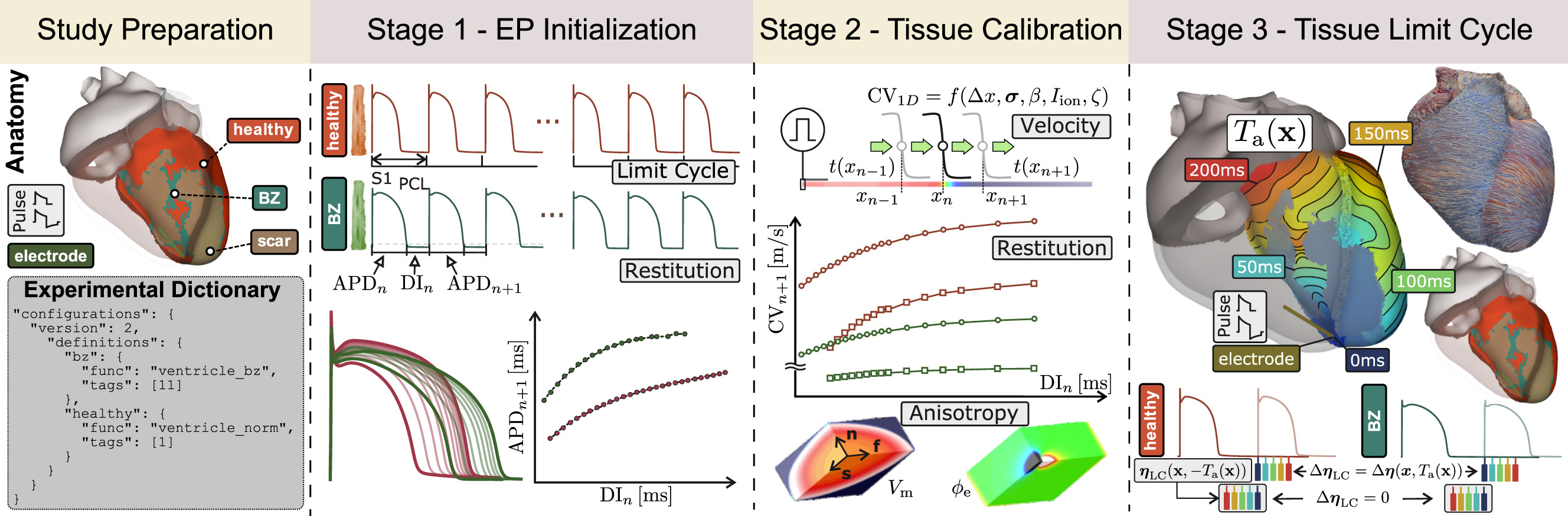
Standardized workflow for electrophysiological simulations contain three main stages as visualized in the figure above:
- Study Preparation: Defining the simulation plan, which includes defining the experimental protocol, the electrophysiological functions, and the solver settings.
- Stage 1 - EP Initialization: Compute the stable limit cycle of all cellular models in the simulation for a given basic cycle length (BCL) and number of beats. Action potential duration (APD) restitution properties are determined and tuned.
- Stage 2 - Tissue Calibration: Tune conductivities to match target conduction velocities for all tissue regions with the given mesh resolution and numerical settings.
- Stage 3 - Tissue Limit Cycle: Initializing all cellular models and tissue properties to reach a stable limit cycle.
Objectives
This example aims to:
- Introduce the concept of simulation plans for defining experimental protocols for the simulation of cardiac electrophysiology.
- Introduce the pipeline of tools present in ForCEPSS for the primary stages in the workflow.
- Showcase the use of ForCEPSS in the implementation of the VARP protocol, which is designed to assess arrhythmia vulnerability in silico.
To access this setup and run through this example, change directories as follows:
cd ${EXAMPLES}/02_EP_tissue/22_forcepss/demoIf you run this example more than once, be sure to replace the plan.json and protocols.json file as it gets overwritten with updated values after execution:
cp ../base_plan.json plan.json
cp ../base_protocols.json protocols.json
Dependencies
The ForCEPSS workflow already available in openCARP consists of the following tools:
- ep_init.py for electrophysiological initialization
- tissue_calibrate.py for tissue calibration
- limit_cycle.py for tissue limit cycle initialization
ForCEPSS depends and actively relies on other openCARP tools:
- limpetgui
- meshalyzer
- bench
- tuneCV
Please make sure all are available and functioning before proceeding!
The ForCEPSS workflow expects the following inputs:
- A discrete computational grid in the form of a mesh suitable for finite element simulations that represents the anatomical structures of interest
- A set of anatomical tags that identify regions within the domain sharing functional properties
- An experimental protocol encoded as a dictionary in JavaScript Object Notation (JSON) format.
Setup
We demonstrate the functionality of ForCEPSS using a 2D tissue patch that replicates settings for the VARP protocol 4 .
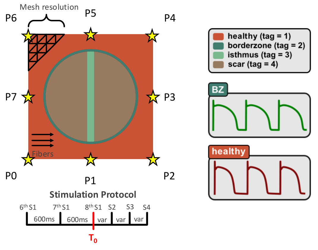
A tissue patch of size 4 cm x 4 cm and average edge length of 0.4 mm was previously generated. Myocardial fibers are incorporated. The tissue has four primary tagged tissue regions to enable reentrant behaviour: healthy (1), borderzone (2), isthmus (3), and scar (4). Each region can be assigned different electrophysiological properties.
For the VARP protocol, the scar is treated as non-conductive bath with an isotropic conductivity of 0.8 S/m. All active tissue regions (healthy, borderzone, and isthmus) were assigned the tenTusscherPanfilov model available in openCARP. For the borderzone and isthmus regions, the following parameter modifications of "GNa*0.38,GCaL*0.31,GKr*0.3,GKs*0.2" were used to replicate the electrophysiological remodelling observed in these regions during myocardial infarction 5 . Conductive properties are provided in the table below. Values are based on those reported in 6 , 7 , and 8 . All tissues are initialized at a BCL of 600 ms.
| Region | Conduction Velocities (m/s) | Conductivities (S/m) |
|---|---|---|
| Healthy | (0.845, 0.4591, 0.4591) | g_il, g_it = (0.255, 0.0775), g_el, g_et = (0.625, 0.236) |
| Borderzone | (0.15, 0.15, 0.15) | g_il, g_it = (0.255, 0.0075), g_el, g_et = (0.625, 0.236) |
| Isthmus | (0.15, 0.15, 0.15) | g_il, g_it = (0.255, 0.0075), g_el, g_et = (0.625, 0.236) |
| Scar | non-conducting | g_bath = 0.8 |
Within the tissue patch, we also assign 8 different locations along the border of the mesh for pacing (P0 - P7) to enable the induction of reentrant behaviour. The locations of the pacing sites are visualized in the figure below. An S1-S2 protocol is used for pacing. Before the pacing protocol, 5 prepacing beats are applied at a BCL of 600 ms to ensure the tissue is in a stable limit cycle before the induction protocol is applied. 20 beats are applied before the premature beat. The start and end coupling intervals for the premature beat are 600 ms and 50 ms, respectively. S2 is decremented by 10 ms until capture. The electrode defintions are defined within the plan.json, while the protocols are defined within protocols.json.
Study preparation
ForCEPSS relies on the concept of simulation plans to define experimental protocols for study preparation in the simulation of cardiac electrophysiology. A simulation plan is a structured definition of the sequence of parameters, protocols, and conditions that govern the execution of a simulation study. The simulation plans are structured as dictionaries and can be saved as json files plan.json. The primary components of a simulation plan include:
- config: defines how element tags are associated with different functional regions
- functions: defines the electrophysiological functions that are used in the simulation (ionic models, conductivities, conduction velocities, etc) for each tissue region.
- solver: defines the underlying components of the solver (time step, tolerances, source models, etc)
- simulation: defines the simulation, including the definition of stimuli/electrodes.
- protocols: defines the experimental protocols that are used in the simulation to induce pacing.
Please look into plan.json and protocols.json for more details on the structure of the simulation plan and how it is used to define the experimental protocol for the VARP protocol.
Stage 1: electrophysiological initialization
EP initialization (often referred to as pre‑pacing) is performed so that the cellular models in each tissue region settle into a stable, repeatable response at a chosen basic cycle length (BCL) after many cycles. In this context, a stable limit cycle means that if you deliver another pacing stimulus at the same BCL, you obtain essentially the same action potential shape and duration, and the key internal state variables (e.g., gating variables, conductances, and ion concentrations) no longer drift from beat to beat. Without EP initialization, early simulation results may therefore reflect transients from arbitrary initial conditions rather than the intended steady behavior at that BCL.
This matters because cells do not instantly respond to a change in pacing or heart rate. Instead, APD adapts over multiple beats when BCL changes, and that adaptation is closely tied to the diastolic interval (DI), i.e., the recovery time between the end of one action potential and the next stimulus. Practically, the relationship is often summarized as BCL ≈ APD + DI. When the pacing rate increases (so BCL decreases), DI typically shortens and APD often shortens as well as there is less time to recover. The relationship between increasing and decreasing BCL/DI and the resultant APD is referred to as an APD resitution curve.
The primary tool for performing this celullar EP initialization, verifying a stable limit cycle, and visualizing APD restitution curves is `ep_init.py`:
ep_init.py --plan                       # Macro parameter experiment description in .json format (simulation plan).
         --bcl                          # Basic cycle length for limit cycle experiment in [ms].
         --cycles                       # Number of cycles to approximated stable limit cycle.
         --update                       # Update ep initial state in experiment description. (default: False)
         --list-funcs                   # List functions on experiment description and exit.
         --restitute                    # Compute restitution curves from limit cycle state. (default:False)
         --plot-apd-restitution         # Plot APD restitution curves. (default:False)
         --apd-restitution-protocol     # APD restitution protocol to use. (default: None)
         --verify                       # Verify limit cycle by comparing state variable traces after cycles offset by 1 cycle.
         --visualize                    # Visualize the results in limpetgui after pacing.
Note that the BCL and number of beats can be defined in the simulation plan, but can also be overridden with command line arguments.
Please refer to the help function for further utility:
ep_init.py --helpRecommended Workflow
Run the following commands to demonstrate how this tool (i) computes a stable limit cycle for the cellular models in each tissue region and (ii) generates APD restitution curves using an S1–S2 protocol.
1.1 Pre-pace each tissue-region cell model
We first pre-pace the cellular model in each tissue region for a fixed number of cycles at the chosen BCL. This allows the state variables (e.g., gating variables, conductances, and ion concentrations) to settle into a steady, repeatable response.
ep_init.py --plan plan.json --cycles 100 --bcl 600 --visualize1.1 Verify that each tissue region is at a stable limit cycle
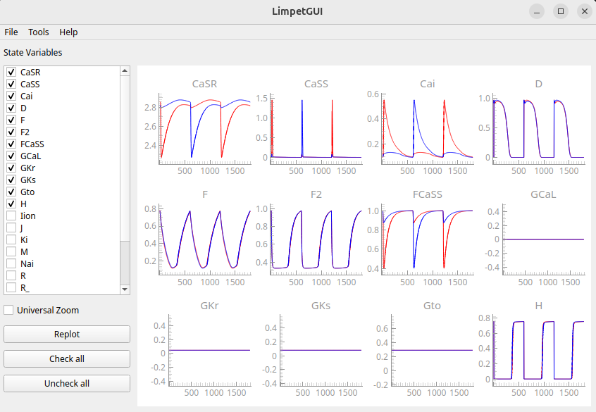
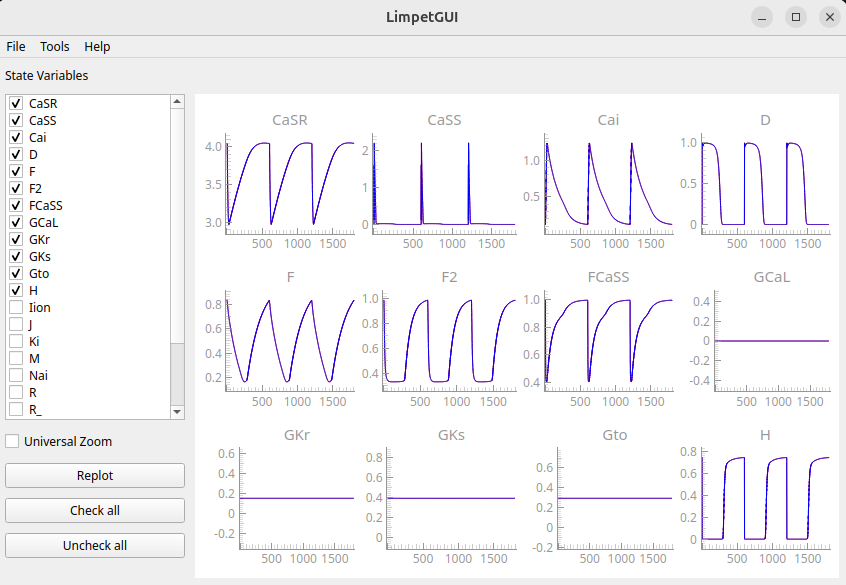
Next, we verify convergence by offsetting by one paced beat (i.e., overlaying consecutive beats). If the models are at a limit cycle, the curves should not change from beat to beat.
ep_init.py --plan plan.json --cycles 100 --bcl 600 --verifyObserve that the BZ is not at steady state after 100 cycles, while the healthy region is:
|
|
1.3 Update the EP initial state in the simulation plan
Once verification is complete, we can update the simulation plan so subsequent runs start from the initialized steady state at this BCL.
ep_init.py --plan plan.json --cycles 100 --bcl 600 --update1.4 Plot APD restitution curves using an S1–S2 protocol
Finally, we compute and plot APD restitution using an S1–S2 protocol. Here DI is interpreted as the recovery time between the end of repolarization and the next stimulus (often approximated as DI ≈ BCL − APD, depending on how APD is measured).
ep_init.py --plan plan.json --restitute --plot-apd-restitution --protocols protocols.json --apd-restitution-protocol s1s2 --updateThe outputted APD restitution curves and restituted APs are visualized in the figures below:
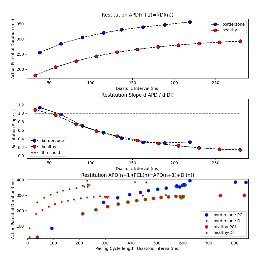
|
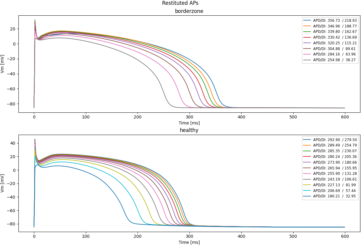
|
Please refer to the example on limpetGUI for more details on the concept of visualizing state variables in the ionic models over cycles at a given BCL.
Stage 2: tissue calibration
The tissue calibration workflow encapsulates establishing limit cycles, measuring CV restitution, tuning conductivities to match targets within tolerance, and reassessing sensitivity to resolution to ensure the calibration holds under your numerical settings.
CV restitution describes how wavefront speed depends on recovery time between activations. Practically, we parameterize recovery by the pacing cycle length (BCL) or, more causally, the diastolic interval (DI), with DI ≈ BCL − APD for a chosen APD definition as introduced above. After conditioning the tissue at each BCL (steady S1 pacing or an S1–S2 probe), CV is measured from activation times. Shorter DI generally yields slower CV because sodium-channel availability and related recovery processes are reduced. Longer DI allows fuller recovery and faster propagation. The result is a CV vs. BCL/DI curve that captures rate dependence. This curve can differ by tissue region and propagation direction in anisotropic media.
In reaction-diffusion simulations, CV is not an input. The CV emerges from the interplay of the conductivity settings, membrane kinetics, tissue structure, and numerics relating to the spatial (dx) and temporal (dt) discretization. Because CV is both emergent and rate dependent, conductivities must be tuned to match target velocities at the intended BCLs and with the specific mesh and solver settings you plan to use. Any change to dx, dt, ionic model, or stimulus protocol can shift the absolute CV and reshape the CV‑restitution curve, so calibration should be performed per tissue region (and per direction, if anisotropic) and verified after changes. Measuring CV restitution ensures the calibrated tissue behaves plausibly across a range of pacing rates in reaction-diffusion simulations.
By contrast, Eikonal‑based methods prescribe CV directly through a speed field (isotropic or anisotropic), so no conductivity tuning is required. You can set the speeds, and activation times follow. This is convenient when the goal is controlled activation timing without detailed ionic dynamics. When physiologic rate dependence really matters, e.g., coupling of APD/DI to propagation, alternans propensity, or interactions between wavefront and ionic state, the reaction-diffusion approach with tuned conductivities may be more appropriate.
The tool encapsulating this stage is `tissue_calibrate.py`:
tissue_calibrate.py --plan              # Macro parameter experiment description in .json format (simulation plan).
         --update                       # Update measured velocities and conductivity settings (if --converge) in simulation plan (default: False)
         --converge                     # Enforce recomputation of conductivities to match given reference conduction velocities. (default: False)
         --c-tol                        # Sets conduction velocity error limit for conduction velocity tuning. (default: 0.0001)
         --resolution                   # Mesh resolution(s) in [um], if given, overrules any resolution settings given in the --plan file.
         --verify                       # Verify limit cycle by comparing state variable traces after cycles offset by 1 cycle.
         --plot-cv-restitution          # Plot CV restitution curve (default: False)
         --restitute-pcl                # List of pacing cycle length for measuring CV restitution (default: None)
         --dx-list                      # List of spatial mesh resolutions in [um] to measure CV for all functional regions given in the --plan file.
         --plot-cv-dx                   # Plot CV dependency on spatial resolution dx. (default: False)
         --tune-mode                    # Select tuning strategy, change gi, gm or beta to obtain prescribed velocities. (default: None)
Note that the resolution can be defined in the simulation plan, but can also be overridden with command line arguments. When using converge, a new set of conductivity values are created in the simulation plan.
The help function contains further utility:
tissue_calibrate.py --helpRecommended workflow
Tissue calibration involves first measuring and plotting CV restitution at a chosen resolution assessing CV against mesh resolution, and then finally converging conductivities to hit target CVs and update the results in the simulation plan. Based on the VARP setup above, we utilize a resolution of 400 microns.
2.1 Plot CV restitution (CV vs BCL)
Use a list of pacing cycle lengths to condition the tissue and measure CV at each BCL.
tissue_calibrate.py --plan plan.json --resolution 400 --plot-cv-restitution --restitute-pcl 600 550 500 450 400 350 300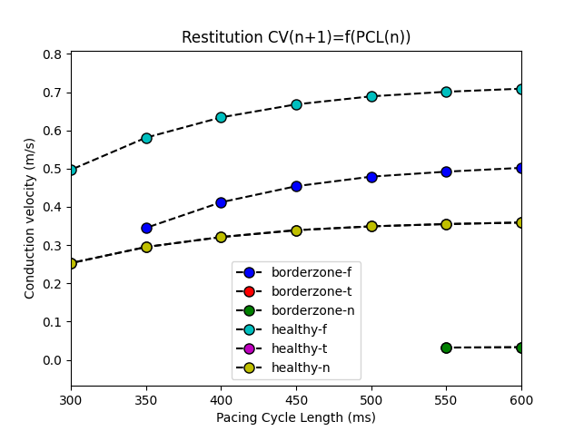
2.2 Plot CV against mesh resolution
Quantify how measured CV depends on spatial resolution to assess numerical sensitivity to spatial discretization of the mesh.
tissue_calibrate.py --plan plan.json --resolution 400 --plot-cv-dx --dx-list 50 100 200 300 400 500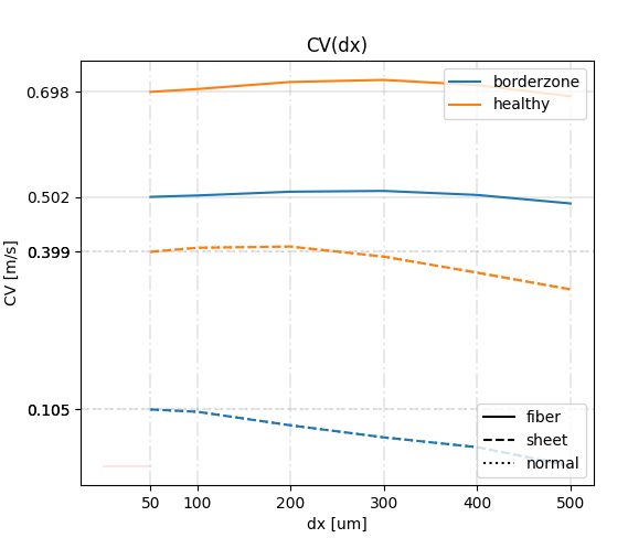
2.3 Converge conductivities to target CVs and update the plan
Iteratively tune conductivities to match reference CVs within tolerance and write the new values back to the simulation plan.
tissue_calibrate.py --plan plan.json --converge --resolution 400 --tune-mode gm --updatePlease refer to the example on tuneCV for more details on the concept of tissue calibration and tuning conduction velocities to match target conduction velocities for all tissue regions with the given mesh resolution and numerical settings.
Stage 3: tissue limit cycle
Before running arrhythmia simulations, it’s important to ensure that both the cellular models and the tissue itself have reached a stable periodic state, or limit cycle. While individual cells can converge to a limit cycle under a given pacing protocol, the behavior of those same cells changes once they are electrically coupled in tissue. Electrotonic loading, wavefront curvature, conduction velocity restitution, and spatial heterogeneities all modify the action potential and conduction properties during the first several beats.
Because of these spatial interactions, tissue often requires additional pre‑pacing cycles to settle into a physiologically consistent rhythm. Achieving this tissue‑scale limit cycle prevents artificial transients from influencing wave propagation, ensures conduction velocity and repolarization gradients are stable, and provides reproducible initial conditions for arrhythmia induction or further physiological simulations.
The tool encapsulating this stage is `limit_cycle.py`:
limit_cycle.py --plan                   # Macro parameter experiment description in .json format (simulation plan).
               --mesh                   # Path and basename of mesh to be prepaced.
               --protocols              # List of protocol descriptions in json format, or within "protocols" section of the simulation plan.
               --protocol               # Pick a specific pre-pacing protocol from protocol list provided through --protocols, or within a "protocols" section in --plan.
               --update                 # Update LAT vector in simulation plan (default: False)
               --stage                  # Select stage: tune for velocities, limit cycle, or validate prepaced state. (default: lim-cyc)
               --electrodes             # List of electrode descriptions in json format or in "electrodes" key in simulation plan.
               --gen-lat                # Generate an activation sequence to create a LAT vector. Choices are ek or rd.
               --lim-cyc                # Select pre-pacing mode to find tissue/organ scale limit cycle.
               --cycles                 # Provide number of cycles to pre-pace (overrules setings in plan/protocol file).
Please refer to the help function for further utility:
limit_cycle.py --helpRecommended workflow
The workflow first applies a pacing protocol to a mesh, then iteratively pre‑paces the tissue until it reaches a stable limit cycle. Once the tissue‑level state is converged and validated, the simulation plan is updated and ready for downstream electrophysiology or arrhythmia studies.
3.1 Pre-pace the tissue using a defined protocol to generate actiation times (LATs)
The protocol described above for prepacing the VARP setup is detailed within protocols.json. We generate the LATs during the firt initial stage.
limit_cycle.py --plan plan.json --mesh ../mesh/istgeom.400um --protocols protocols.json --protocol lcP0 --stage gen-lat --gen-lat ek --update --visualize3.2 Compute limit cycle using the computed activation sequence
Now that the plan.json has been updated with the protocols, we can proceed without specifying the json file directly.
limit_cycle.py --plan plan.json --mesh ../mesh/istgeom.400um --protocol lcP0 --stage lim-cyc --lim-cyc lat-2 --visualize3.3 Do same process for all other electrodes (P1-P7)
limit_cycle.py --plan plan.json --mesh ../mesh/istgeom.400um --protocol lcP1 --stage gen-lat --gen-lat ek --update --visualize

limit_cycle.py --plan plan.json --mesh ../mesh/istgeom.400um --protocol lcP1 --stage lim-cyc --lim-cyc lat-2
You are now ready to start your simulations using the generated checkpoints!
References
Gsell MAF, Neic A, Bishop MJ, Gillette K, Prassl AJ, Augustin CM, Vigmond EJ, Plank G. ForCEPSS—A framework for cardiac electrophysiology simulations standardization. Computer Methods and Programs in Biomedicine, 251, 108189 (2024). DOI: 10.1016/j.cmpb.2024.108189↩︎
Arevalo HJ, Vadakkumpadan F, Guallar E, Jebb A, Malamas P, Wu KC, Trayanova NA. Arrhythmia risk stratification of patients after myocardial infarction using personalized heart models. Nature Communications, 7, 11437 (2016). DOI: 10.1038/ncomms11437↩︎
Arevalo HJ, Vadakkumpadan F, Guallar E, Jebb A, Malamas P, Wu KC, Trayanova NA. Arrhythmia risk stratification of patients after myocardial infarction using personalized heart models. Nature Communications, 7, 11437 (2016). DOI: 10.1038/ncomms11437↩︎
Gsell MAF, Neic A, Bishop MJ, Gillette K, Prassl AJ, Augustin CM, Vigmond EJ, Plank G. ForCEPSS—A framework for cardiac electrophysiology simulations standardization. Computer Methods and Programs in Biomedicine, 251, 108189 (2024). DOI: 10.1016/j.cmpb.2024.108189↩︎
Arevalo HJ, Vadakkumpadan F, Guallar E, Jebb A, Malamas P, Wu KC, Trayanova NA. Arrhythmia risk stratification of patients after myocardial infarction using personalized heart models. Nature Communications, 7, 11437 (2016). DOI: 10.1038/ncomms11437↩︎
Costa CM, Gemmell P, Elliott MK, Whitaker J, Campos FO, Strocchi M, Neic A, Gillette K, Vigmond E, Plank G, Razavi R, O'Neill M, Rinaldi CA, Bishop MJ. Determining anatomical and electrophysiological detail requirements for computational ventricular models of porcine myocardial infarction. Computers in Biology and Medicine, 141, 105061 (2022). DOI: 10.1016/j.compbiomed.2021.105061↩︎
Recent questions tagged experiments, tissue, reentry, pacing, forcepss
There are tagged with experiments, tissue, reentry, pacing, forcepss.
Here we display the 5 most recent questions. You can click on each tag to show all questions for this tag.
You can also ask a new question.