Eikonal Example

See code in GitLab.
Author: Cristian Barrios Espinosa cristian.espinosa@kit.edu, Tobias Gerach tobias.gerach@kit.edu

Eikonal Simulations

Eikonal simulations in openCARP provide a computationally efficient way to calculate activation times from electrical wave propagation in cardiac tissue. These simulations do not model transmembrane voltage dynamics, making them ideal for fast approximations or pre-analysis steps.

To run the experiments of this example, navigate to:

cd ${TUTORIALS}/03_Eikonal/01_Eikonal

Eikonal Simulation Setup

To perform an eikonal simulation, the regions in the mesh must be assigned to a physics region of type eikonal. The following code extracts the intracellular element tags and configures the physics options:

_, etags, _ = txt.read(meshname + '.elem')
etags = np.unique(etags)
IntraTags = etags[etags != 0].tolist()

print('IntraTags:', IntraTags)

phys_opts = tools.gen_physics_opts(EikonalTags=IntraTags)
cmd += phys_opts

To ensure the solver runs in pure eikonal mode, configure the simulation parameters as follows:

dream.solve = 0
dream.fim.max_iter = 10000000
dream.fim.tol = 0.001

Here, dream.solve = 0 determines which method is used to solve the eikonal equation. Method 0 uses the fast iterative method (FIM) to calculate activation times. The remaining parameters are tuned for efficient convergence of the FIM algorithm. Typically, larger more complex meshes require more FIM iterations. Therefore, if you still see activation time values of -1 in the solution file act.igb you need to increase dream.fim.max_iter. The precision of the solutions of FIM is determined by dream.fim.tol.

Usage

The run.py script exposes a variety of parameters for easy experimentation. Use:

python3 run.py --help
...
Tutorial specific options:
 --dx DX                                 Resolution of the mesh in um. (default: 1000.0)
 --elemType {tetra,tri}                  Defines if 2D or 3D mesh is created. (default: tetra)
 --cv CV                                 Set conduction velocity in mm/s in fiber direction. (default: 500.0)
 --ar AR                                 Set anisotropy ratio perpendicular to fiber direction. (default: 1.0)
 --mesher [{sphere,box} ...]             Add regional heterogeneity to the mesh. (default: [])
 --fiber_orientation FIBER_ORIENTATION   Set a fiber orientation angle. (default: 0)

to display all available options and default values. Running the script with the parameter --visualize will open the activation time file in meshalyzer after the simulation is done. In case of a 3D simulation, you first have to generate a surface in meshalyzer.

Experiments

This tutorial uses a simple 2D slab or 3D block geometry to demonstrate different wavefront propagation scenarios under various conduction velocities, anisotropy ratios, and fiber orientations.

Experiment 1: Isotropic Radial Activation

Run the simplest simulation: isotropic conduction with a radial wavefront.

python3 run.py --visualize --elemType tri --ar 1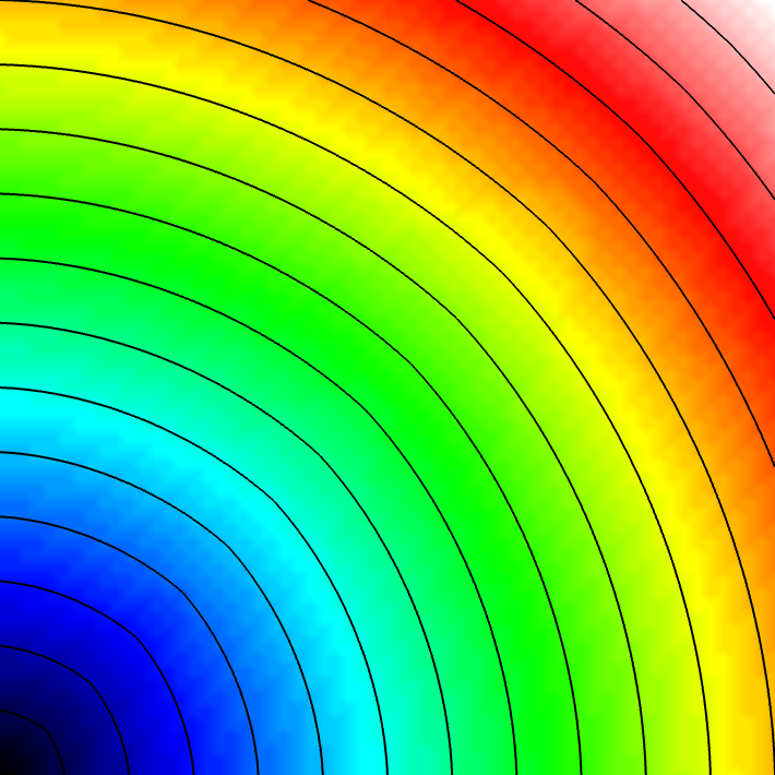

Experiment 2: Anisotropic Radial Activation

Modify the anisotropy ratio using the --ar parameter (longitudinal to transverse conduction velocity).

python3 run.py --visualize --elemType tri --ar 3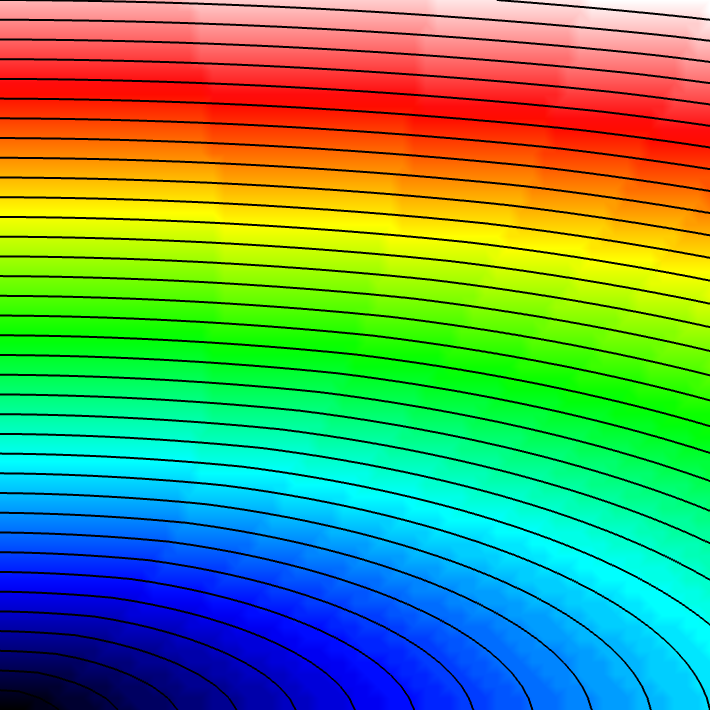

Experiment 3: Tilted Fiber Orientation

Alter the propagation direction by changing the fiber orientation.

python3 run.py --visualize --elemType tri --ar 3 --fiber_orientation 60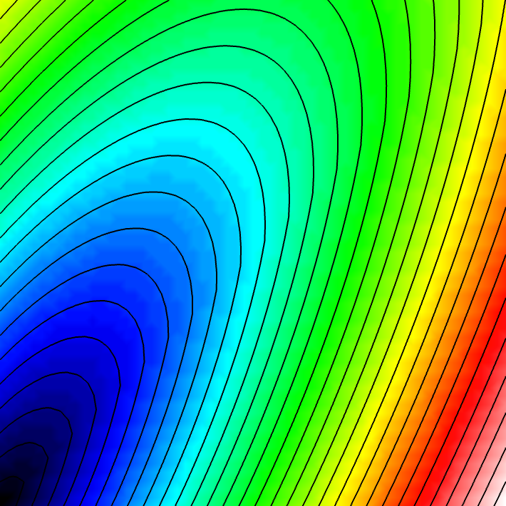

Experiment 5: Heterogeneous Conduction Regions

Introduce heterogeneity by reducing conduction velocity in different regions. You can use sphere and box individually as well.

python3 run.py --visualize --elemType tri --ar 1 --mesher sphere box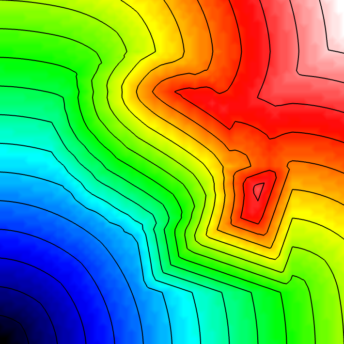

Experiment 6: 3D simulations

Run simulation in a 3D block with tetrahedral elements. Works with combinations of the other experiments as well.

python3 run.py --visualize --elemType tetra --ar 1 --mesher sphere box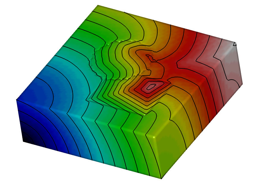

Recent questions tagged experiments, examples, tissue, eikonal