Reaction Eikonal Example

See code in GitLab.
Author: Cristian Barrios Espinosa cristian.espinosa@kit.edu

Introduction

Reaction-eikonal simulations in openCARP provide a computationally efficient way to calculate transmembrane voltages at a low computational cost by using coarse meshes [neic2017].

To run the experiments of this example, navigate to:

cd ${TUTORIALS}/03_Eikonal/02_Reaction_Eikonal

Simulation Setup

To perform a reaction-eikonal simulation, the regions in the mesh geometry must be assigned to a physics region of type eikonal. The following code extracts the intracellular element tags and configures the physics options:

_, etags, _ = txt.read(meshname + '.elem')
etags = np.unique(etags)
IntraTags = etags[etags != 0].tolist()

print('IntraTags:', IntraTags)

phys_opts = tools.gen_physics_opts(EikonalTags=IntraTags)
cmd += phys_opts

To ensure the solver runs in reaction-eikonal mode, configure the simulation parameters as follows:

dream.solve = 1|2
dream.fim.max_iter = 10000000
dream.fim.tol = 0.001

Here, dream.solve = 2 ensures that RE- is computed whereas with dream.solve = 1 RE+ is computed adding the real diffusion current. Method 0 uses the fast iterative method (FIM) to calculate activation times. The remaining parameters are tuned for efficient convergence of the FIM algorithm. Typically, larger more complex meshes require more FIM iterations. Therefore, if you still see activation time values of -1 in the solution file act.igb you need to increase dream.fim.max_iter. The precision of the solutions of FIM is determined by dream.fim.tol.

Experiments

This tutorial uses a simple 2D slab with different wavefront propagation scenarios using various conduction velocities.

Experiment 1: Anisotropic Radial Activation RE- (Activation Times)

Run the simplest simulation: radial propagation stimulating a point in the left side of the Slab and with a bit of delay in the bottom right corner. Use the --visualize_mode 1 to visualize the activation times in meshalyzer.

python3 run.py --visualize_mode 1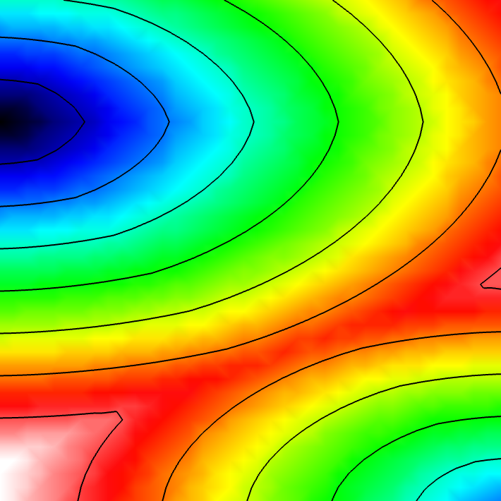

Note that the simulation was run in a mesh with triangular elements with an average edge lenth of 800 um, which would be unfeasible in monodomain simulations due to numerical artifacts.

Experiment 2: Anisotropic Radial Activation RE- (Transmembrane Voltages)

Modify the running time of the simulation using --tend to see the repolarization phase and set --visualize_mode 2 to observe the transmembrane voltage (longitudinal to transverse conduction velocity).

python3 run.py --visualize_mode 2 --tend 500

Experiment 3: Heterogeneous Conductivities

It is possible to run a simulation defining heterogenous conduction velocity with different ionic model parameters in the RE- model.

python3 run.py --visualize_mode 2 --tend 500 --heterogeneous 1

To improve the gradients of transmembrane voltage during repolarization, it is better to use RE+ by setting --solve 1. It is important to note that in case of the RE+ model, the approximation of the diffusion current guarantees a latest activation time of the myocardium, but activation can happen earlier due to real diffusion currents. Hence, a combination of velocities (vel_l, vel_t, vel_n) and conductivities (g_l, g_t, g_n) must be identified that yields the desired conduction velocity in the myocardium. To do so, we use the tuneCV utility of carputils to obtain matching CV and conductivity values. Otherwise, the activation times due to diffusion currents diverge from the eikonal based arrival times.

python3 run.py --visualize_mode 2 --tend 500 --heterogeneous 1 --solve 1

Recent questions tagged experiments, examples, tissue, eikonal