DREAM pacing simulation example

See code in GitLab.
Author: Tobias Gerach tobias.gerach@kit.edu

This example demonstrates how to use the Diffusion Reaction Eikonal Alternant Model (DREAM). To run the experiments of this example, navigate to:

cd ${TUTORIALS}/03_Eikonal/03B_DREAM_pacing

Introduction

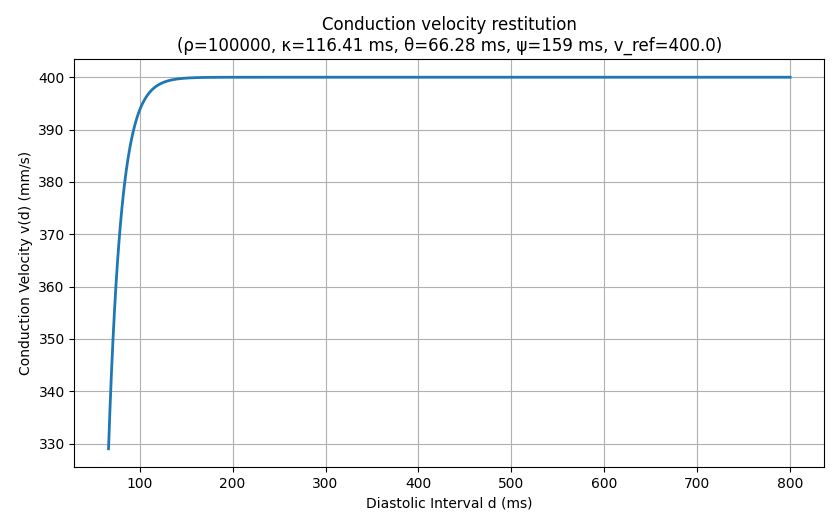
In this example, we will explore how the Diffusion Reaction Eikonal Alternant Model (DREAM) behaves during pacing protocols. During pacing protocols, an important characteristic of cardiac tissue is restitution. For the DREAM, we want to look at conduction velocity (CV) restitution in particular. Typically, CV reduces when the pacing frequency is increased.

Conduction velocity restitution used in this tutorial. The parameters are for the Courtemanche ionic model including remodelling during atrial fibrillation [Barrios2024].

Data output

Unlike the Eikonal and Reaction-Eikonal model, the DREAM runs in a cyclical manner, i.e. the eikonal equation is solved multiple times in alteration with the reaction part of the parabolic system. Therefore, the .igb files for activation and repolarization times is updated in cycles as well. Saving this data as .igb files has the advantage that you can easily visualize these files in meshalyzer. However, you have to interpret the typical time step slider as eikonal computation cycles instead. I recommend to set the color scale to auto if you do this. Another advantage is that you can use the IGB tools in carputils to postprocess these files however you want. If you are more interested in the local activation times based on transmembrane voltages, you can still use the traditional way of detecting activation times in openCARP by using the LAT sentinel.

Problem setup

Mesh

First, we build a geometry for this experiment using mesher. The mesh is a simple 80mm by 50mm slab, which is discretized using triangles.

Ionic model

This tutorial uses the Courtemanche ionic model for human atrial myocytes [Courtemanche1998]. We use a version of the model with modified ion channel conductances using the -imp_region[].im_param parameter according to [Loewe2016]. To switch between a healthy and AF parameterization, use the option --AF or --no-AF, respectively.

Pacing protocol

We apply a stimulus on the left edge of the mesh. With the option --bcl, the user can set the basic cycle length. The number of cycles is set to 3.

Usage

The following optional arguments are available (default values are indicated):

python3 ./run.py --help
...
Tutorial specific options:
--dx DX               Set resolution of the mesh in um (default: 1000.0)
--cv CV               Set conduction velocity in mm/s in fiber direction (default: 400.0)
--ar AR               Set anisotropy ratio perpendicular to fiber direction. (default: 1.0)
--bcl BCL             Set the basic cycle length for the stimulation. (default: 250)
--model {0,1,2,3}     Choose model to solve: Eikonal(0), RE+(1), RE-(2), DREAM(3) (default: 3)
--tau_inc TAU_INC     Maximum allowed increment of minimum activation time in every DREAM cycle. (default: 100.0)
--AF, --no-AF         Determine if you want to use Courtemanche with remodelled ionic channels (--AF) or using the default
                      Courtemanche (--no-AF). (default: None)

After running the script, activation time, repolarization time, diffusion current and transmembrane voltage are output to the files act.igb, rpt.igb, idiff.igb, and vm.igb, respectively. Running the script with the parameter --visualize will open the transmembrane voltage file in meshalyzer after the simulation is done.

Tasks

Familiarize yourself with the output of the DREAM by visualizing activation times, repolarization times, and transmembrane voltage using meshalyzer.

2. Using our simple 2D mesh in an isotropic setting, we can calculate the activation times that are solutions to the eikonal equation with the relation \(t = d/v\), where d is the distance travelled and v is the CV. Since we simulate a planar wavefront, the distance d is 80 mm at the right edge of the mesh. Using a CV of 400 mm/s, this should result in an activation time of 200 ms for the first stimulus. Confirm this result by running the corresponding simulation with a BCL of 300 ms and the --AF option.

How does the travel time (activation time - stimulus time) on the right edge change for the 2nd and 3rd stimulation if you use a BCL of 150 ms?

4. Use the same runtime options as in task 2. What happens if you additionally set --tau_inc to 300ms?

Solutions to the tasks

Simply running the following command will visualize the transmembrane voltage in meshalyzer.

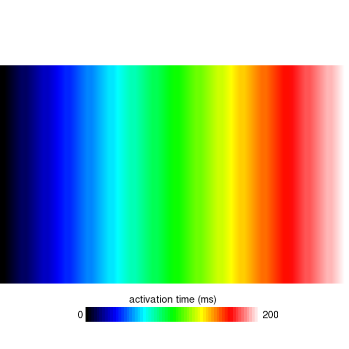
python3 run.py --visualize

Everything should be as know it from bidomain or monodomain simulations. To open the eikonal activation times, click on File, Read Data and navigate to the directory eik_3_AF to open the file act.igb. Set the color scale to auto for best viewing and scroll through the eikonal cycles using the time slider. You should see something like this:

Visualization of activation times in the different eikonal cycles from task 1. Values of -1 mean the region was not activated yet.

Similarly, you can visualize the repolarization times which are calculated when Vm crosses the threshold set by the dream parameter dream.repol_time_thresh.

Using the command

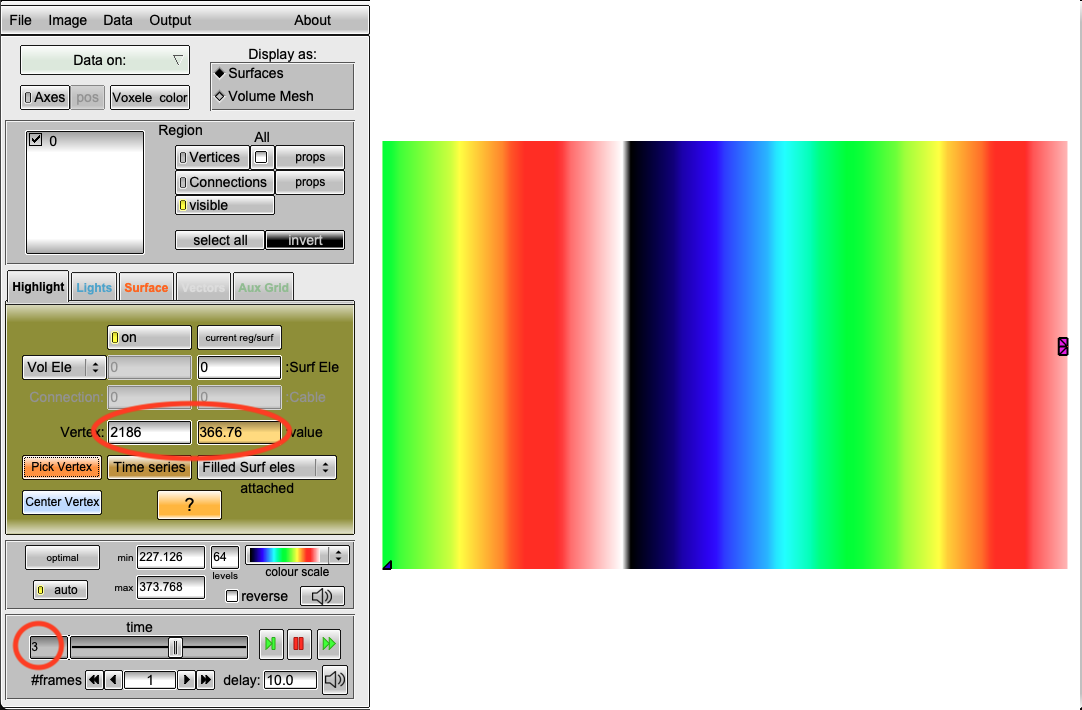
python3 run.py --visualize --cv 400 --bcl 300 --AF

we can open the file act.igb as described in the solution to task 1. As shown in the following figure, you should find that in cycle 1, the activation time on the right edge of the mesh is 200ms. You will find that the same holds true for the 2nd and 3rd stimulus by looking at cycles 3 and 5, respectively.

Visualization of activation times in the first (==1) eikonal cycle from task 2. The maximum time is 200ms at the right edge.

Using the command

python3 run.py --visualize --cv 400 --bcl 150 --AF

we can open the act.igb file and look at the 1st, 3rd, and 5th eikonal cycle. In the 1st cycle, we can still observe a travel time of 200ms. However, in the 3rd and 5th cycle we find \(366.76-150 = 216.76\) ms and \(512.98-300 = 212.98\) ms, respectively. Clearly, the conduction velocity is lower (approx. 377mm/s) after the second and third stimulus. This is expected and a result of the DREAM adhering to the CV restitution curve shown in the beginning.

Visualization of activation times in the thrid (==3) eikonal cycle from task 3. The activation time at the right edge of the mesh is 366.76ms shown by the examplary node with ID 2186.

Using the command

python3 run.py --visualize --cv 400 --bcl 300 --AF --tau_inc 300

you will notice that the second stimulus is missing. The DREAM parameter tau_inc essentially sets how far the eikonal solutions can advance in time based on the smallest calculated activation time of the current cycle. Therefore, the second stimulus will be skipped in certain scenarios. In this case it is skipped, because all nodes converge before the second stimulus is applied and the reaction part is allowed to advance too far. On a much larger mesh, this might not have been a problem. A good rule of thumb is to choose tau_inc smaller than half of you BCL.