DREAM reentry simulation example

See code in GitLab.
Author: Tobias Gerach tobias.gerach@kit.edu

cd ${TUTORIALS}/03_Eikonal/03B_DREAM_reentry

Introduction

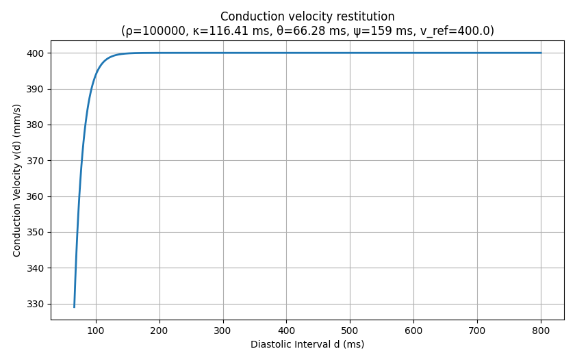
In the Diffusion Reaction Eikonal Alternant Model (DREAM) the possibility of simulating a reentry is given, since it uses the cyclical fast iterative method to compute activation times from the eikonal equation [Barrios2024]. In each iteration, converged nodes are allowed to be activated again if they fullfil certain conditions. These conditions involve the repolarization time of the individual cell at each node. The most important condition that is relevant for the user is that the DREAM uses conduction velocity restitution based on the diastolic interval. This makes it possible to respect the refractory state of the cell and to reflect the typical behavior of cardiac tissue during pacing, i.e. a reduced conduction velocity when pacing frequency is increased. By default, conduction velocity restitution in DREAM is calculated by the formula

\[v(d) = v_\mathrm{ref} \cdot \left( 1 - \rho \cdot \exp(-\frac{\log(\rho)}{\psi} (d + \kappa))\right)\]

if \(d > \theta\), where d is the diastolic interval and v is conduction velocity. Therefore, \(\theta\) determines a cutoff below which conduction is not possible anymore, since we are inside the refractory phase of the cell.

Problem setup

Mesh

First, we build a geometry for this experiment using mesher and the dynamic retagging feature of openCARP. The mesh is a simple 60mm by 60mm slab, which is discretized using triangles. In the centre of this mesh, we place a spherical region with elemTag = 2. Later, this will represent a non_conductive region with a conduction velocity of 0. With dynamic retagging, we place a conductive channel through the middle of this spherical region with elemTag = 3. By default, the mesh resolution is set to \(1000 \mu m\), but you can change it during runtime with the parameter --dx.

Ionic model

This tutorial uses the Courtemanche ionic model for human atrial myocytes [Courtemanche1998]. Since we want to simulate a reentry, we modify ion channel conductances using the -imp_region[].im_param parameter according to [Loewe2016] to include remodelling during atrial fibrillation. To switch between a healthy and AF parameterization, use the option --AF or --no-AF, respectively.

Pacing protocol

We use a simple S1-S2 protocol to induce a reentry. The S1 stimulus is applied on the left edge of the 2D slab. The S2 stimulus is applied to a cluster of nodes 4mm around the coordinate (9, 30, 0)mm and the time is set by the user using the parameter --S2 XXX with XXX being the cycle length after the S1 start time.

Usage

The following optional arguments are available (default values are indicated):

python3 ./run.py --help
...
Tutorial specific options:
  --dx DX               Set resolution of the mesh in um (default: 1000.0)
  --cv CV               Set conduction velocity in mm/s in fiber direction (default: 400.0)
  --ar AR               Set anisotropy ratio perpendicular to fiber direction. (default: 1.0)
  --model {0,1,2,3}     Choose model to solve: Eikonal(0), RE+(1), RE-(2), DREAM(3) (default: 3)
  --S2 S2               Set start time of S2 stimulus (default: None)
  --plotCVrest          Plot CV restitution properties (default: False)
  --AF, --no-AF         Determine if you want to use Courtemanche with remodelled ionic channels (--AF) or using the default
                        Courtemanche (--no-AF). (default: None)

After running the script, activation time, repolarization time, diffusion current and transmembrane voltage are output to the files act.igb, rpt.igb, idiff.igb, and vm.igb, respectively. Running the script with the parameter --visualize will open the transmembrane voltage file in meshalyzer after the simulation is done.

Tasks

1. Use the CV restitution properties provided above to determine an S2 stimulus time that induces a reentry.

2. Can you determine an S2 stimulus time for which a reentry is possible using the standard model parameters of Courtemanche? Use the option --no-AF to turn AF parameterization off.

Solutions to the tasks

1. According to the provided CV restitution, the minimum diastolic interval at which a stimulus can be propagated is 66.28ms. Therefore, you can check the repolarization time (RT) of the nodes to the right of the S2 stimulus (node ID 1839) in the output file rpt.igb. Choose your S2 stimulus time such that a propagation to the right is blocked but a propagation to the left is possible. For example, the repolarization time at the point with ID 1840 is 110.575ms, meaning every propagation until approx. 176ms will be blocked. Therefore, one possible solution is

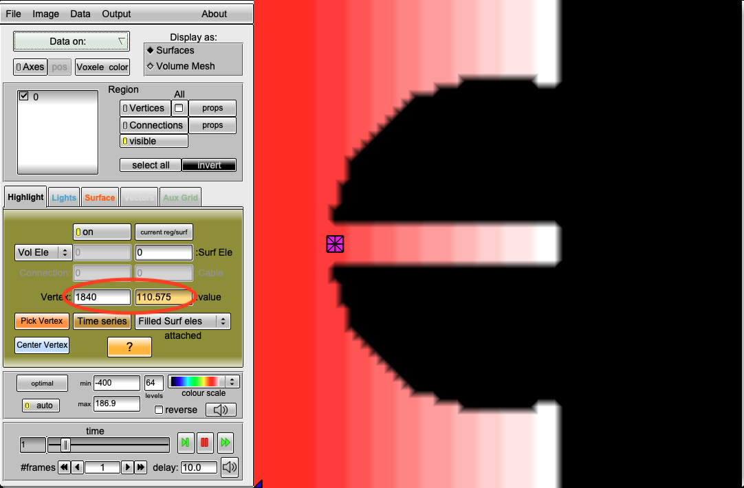
python3 run.py --visualize --S2 175 --AF

2. We can approach this in the same manner as task 1. However, the default parameterization of the Courtemanche model leads to a longer action potential duration and the repolarization time at point 1840 is now 208.075ms. Using the --plotCVrest and --no-AF together will show you that we now require an S2 stimulus time of less than 345ms for it to be blocked (sometimes 5ms more are still sufficient). As we will see, this will initially result in a propagation block to the right side of the stimulus but not in a stable reentry, since it is blocked from propagation at a later time. Therefore, without changing other parameters such as CV, the answer is no. We can not induce a reentry with the given protocol using the default Courtemanche model! Command to generate the figures:

python3 run.py --visualize --no-AF --S2 345

Recent questions tagged experiments, examples, tissue, eikonal