Adjusting parameters (wavelength) to experimental data
See code in GitLab.
Author: Jason Bayer jason.bayer@ihu-liryc.fr
This example demonstrates how to adjust parameters in tissue simulations to match experimental data for conduction velocity, action potential duration, and wavelength. To run the experiments of this example change directories as follows:
cd ${EXAMPLES}/02_EP_tissue/03C_tuning_wavelengthIntroduction
It is important that computer simulations in cardiac tissue corroborate experimental data. In particular, conduction velocity (CV) is the speed at which electrical waves propagate in cardiac tissue, and action potential duration (APD) is the time duration a cardiac myocyte repolarizes after excitation. The multiplication of CV and APD is termed the wavelength for reentry (\(\lambda\)), which is the minimum length cardiac tissue dimensions have to be in order to support reentry from unidirectional conduction block. In this exercise, the user will perform a basic example of how to adjust CV and APD in a 2D cardiac sheet of ventricular tissue to match CV and APD from experimental data recorded on the ventricular epicardium of human ventricles with optical imaging.
Problem setup
To execute simulations of this example do
cd ${EXAMPLES}/02_EP_tissue/03C_tuning_wavelengthExperimental data
The mapping of electrical activity with optical imaging on the epicardium of human ventricles provides an accurate measurement of CV 1 and APD 2 . The data from these studies is shown below and were recorded during baseline pacing with a cycle length of 1000 ms.
|
\(CV_\mathrm{l}\) (cm/s) | \(CV_\mathrm{t}\) (cm/s) | \(APD_{80}\) (ms) | \({\lambda}_\mathrm{l}\) (cm) | \({\lambda}_\mathrm{t}\) (cm) |
|---|---|---|---|---|---|
|
|
|
|
|
|
1D cable model
A 1.5 cm cable of epicardial ventricular myocytes is used to initially adjust CV and APD to experimentally derived values. The model domain was discretized with linear finite elements with an average edge length of 0.02 cm.
2D sheet model
A 1.5 cm x 1.5 cm sheet of epicardial tissue is used to verify CV and APD derived in the 1D cable model. The model domain is discretized using quadrilateral element finite elements with an average edge length of 0.02 cm, and a longitudinal fiber direction in each element parallel to the X-axis of the sheet. The mesh was generated using the command below according to the mesher tutorial.
mesher -size[0] 1.5 -size[1] 1.5 -size[2] 0.0 -resolution[0] 200.0 -resolution[1] 200.0 -resolution[2] 0.0Ionic model
For this example, we use the most recent version of the ten Tusscher ionic model for human ventricular myocytes 3 . This ionic model is labeled tenTusscherPanfilov in openCARP's LIMPET library. After a quick literature search, one will find that the slow outward rectifying potassium current \(I_{K_{s}}\) is heterogeneous across the human ventricular wall 4 . Therefore, the maximal conductance \(G_{K_{s}}\) of \(I_{K_{s}}\) is adjusted in order to match the APD=340 ms derived experimentally. Note, the default value for \(G_{K_{s}}\) in epicardial ventricular myocytes is 0.392 nS/pF.
Pacing protocol
The left side of the 1D cable model and the center of the 2D sheet model is paced with 5-ms-long stimuli at twice capture amplitude for a cycle length and number of beats chosen by the user.
Conduction velocity
To determine initial conditions for the tissue conductivities along (\(\\sigma_{\\mathrm{il}}\), \(\\sigma_{\\mathrm{el}}\)) and transverse (\(\\sigma_{\\mathrm{it}}\), \(\\sigma_{\\mathrm{et}}\)) the fibers in the models, tuneCV is used as described in the example Tuning Conduction Velocities. The commands to obtain the two conductivities are listed below.
tuneCV --converge true --tol 0.0001 --velocity 0.92 --model tenTusscherPanfilov --sourceModel monodomain --resolution 200.0

tuneCV --converge true --tol 0.0001 --velocity 0.22 --model tenTusscherPanfilov --sourceModel monodomain --resolution 200.0
The initial conductivities resulting from tuneCV are \(\\sigma_{\\mathrm{il}}=0.4134\) S/m, \(\\sigma_{\\mathrm{el}}=1.4849\) S/m, \(\\sigma_{\\mathrm{it}}=0.0379\) S/m, and \(\\sigma_{\\mathrm{et}}=0.1361\) S/m.
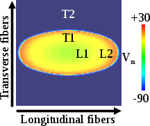
To compute CV, activation times are computed for the last beat of the pacing protocol using the openCARP option LATs (see example on electrical mapping), with activation time recorded at the threshold crossing of -10 mV. CV is then computed along the cable by taking the difference in activation times at the locations 1.0 cm and 0.5 cm divided by the distance between the two points. For the sheet model, CV is computed along the longitudinal and transverse fiber directions by taking the difference in activation times at the locations illustrated in the figure below. Specifically, \(CV_{l}\) = 0.25/(L2-L1) and \(CV_{t}\) = 0.25/(T2-T1). The locations of L1 and T1 are 0.25 cm away from the tissue center, and L2 and T2 are 0.5 cm away from the tissue center.
Action potential duration
Action potential duration is computed at 80% repolarization (\(APD_{80}\)) according to [Bayer2016]. This is achieved by using the igbutils function igbapd as illustrated below (replace ./vm.igb with the proper location of your file).
igbapd --repol=80 --vup=-10 --peak-value=plateau ./vm.igb Usage
The following optional arguments are available (default values are indicated):
./run.py --help
  --dimension         Options: {cable,sheet}, Default: cable
                      Choose cable for quick 1D parameter adjustments,
                      then the 2D sheet to verify the adjustments.
  --GKs               Default: 0.392  nS/pF
                      Maximal conductance of IKs
  --Gil               Default: 0.3544 S/m
                      Intracellular longitudinal tissue conductivity
  --Gel               Default: 1.27 S/m
                      Extracellular longitudinal tissue conductivity
  --Git               Default: 0.024 S/m
                      Intracellular transverse tissue conductivity
  --Get               Default: 0.0862 S/m
                      Extracellular transverse tissue conductivity
  --nbeats            Default: 3
                      Number of beats for pacing protocol. This number
                      should be much larger to achieve steady-state
  --bcl               Default: 1000
                      Basic cycle length for pacing protocol
  --times             Default: 1000
                      Time before applying pacing protocol
After running run.py, the results for APD, CV, and (\(\\lambda\)) can be found in the file adjustment_results.txt within the output subdirectory for the simulation.
If the program is ran with the --visualize option, meshalyzer will automatically load the \(V_\\mathrm{m}(t)\)
for the last beat of the pacing protocol. Output files for activation and APD are also produced for each
simulation and can be found in the output directory and loaded into meshalyzer.
Tasks
- Determine the value for IKs to obtain the experimental value for APD in the cable.
- Place this value in the sheet model to verify the model is behaving in the same manner as the simple cable model.
- Determine a set of Gil and Gel (keep ratio for Gil/Git the same) so that both the longitudinal and transverse wavelengths are less than 8 cm.
Solutions to the tasks
- A GKs=0.22 nS/pF is needed to obtain the APD of about 340 ms.
./run.py --GKs 0.22 --dimension cable- The following command produces a similar APD in the sheet model.
./run.py --GKs 0.25 --dimension sheet- The following commands produce longitudinal and transverse wavelengths less than 8 cm.
./run.py --GKs 0.25 --Gil 0.02 --Git 0.0135 --dimension cable

./run.py --GKs 0.25 --Gil 0.02 --Git 0.0135 --dimension sheet
References
Glukhov AV, Fedorov VV, Kalish PW, Ravikumar VK, Lou Q, Janks D, Schuessler RB, Moazami N, Efimov IR. Conduction remodeling in human end-stage nonischemic left ventricular cardiomyopathy. Circulation, 125(15):1835-1847, 2012. DOI: 10.1161/CIRCULATIONAHA.111.047274↩︎
Glukhov AV, Fedorov VV, Lou Q, Ravikumar VK, Kalish PW, Schuessler RB, Moazami N, and Efimov IR. Transmural dispersion of repolarization in failing and nonfailing human ventricle. Circ Res, 106(5):981-991, 2010. DOI: 10.1161/CIRCRESAHA.109.204891↩︎
ten Tusscher, K. H. W. J. & Panfilov, A. V., Alternans and spiral breakup in a human ventricular tissue model, Am. J. Physiol. Heart Circ. Physiol. 291, H1088-H1100, 2006. DOI: 10.1152/ajpheart.00109.200↩︎
Pereon Y, Demolombe S, Baro I, Drouin E, Charpentier F, Escande D. Differential expression of kvlqt1 isoforms across the human ventricular wall. Am J Physiol Heart Circ Physiol, 278(6):H1908-H1915, 2000. DOI: 10.1152/ajpheart.2000.278.6.H1908↩︎
Recent questions tagged experiments, examples, tunecv, tissue
There are tagged with experiments, examples, tunecv, tissue.
Here we display the 5 most recent questions. You can click on each tag to show all questions for this tag.
You can also ask a new question.