Simplified Kirchhoff network coupling

See code in GitLab.
Author: Moritz Linder moritz.linder@kit.edu, Michele Terren michele.terren@studio.unibo.it

Overview

cd ${EXAMPLES}/04_sknm_tissue/01_sknm_san 

This example demonstrates how individual cell models sampled from a population of models (POMs) can be discretely coupled using the simplified Kirchhoff network model (SKNM) and simulated within a small tissue patch. Specifically, the SKNM provides an alternative coupling strategy that lies between the homogenised mono- and bidomain formulations and the extracellular-membrane-intracellular (EMI) model, which explicitly resolves individual myocytes and the surrounding extracellular space. More information about the POMs can be found in the Parallel single-cell simulations example.

Problem definition

While single-cell models provide valuable insights into the electrophysiological behaviour of isolated cells, they cannot reproduce complex physiological phenomena such as action potential propagation, nor pathological dynamics such as re-entries, which emerge at tissue level. To investigate these processes, several modelling strategies have been developed to simulate tissue, ranging from small tissue patches to whole-heart models. These approaches can be broadly categorised as spatial models and, as illustrated in Figure 1, represent cardiac tissue at different levels of detail and computational costs.

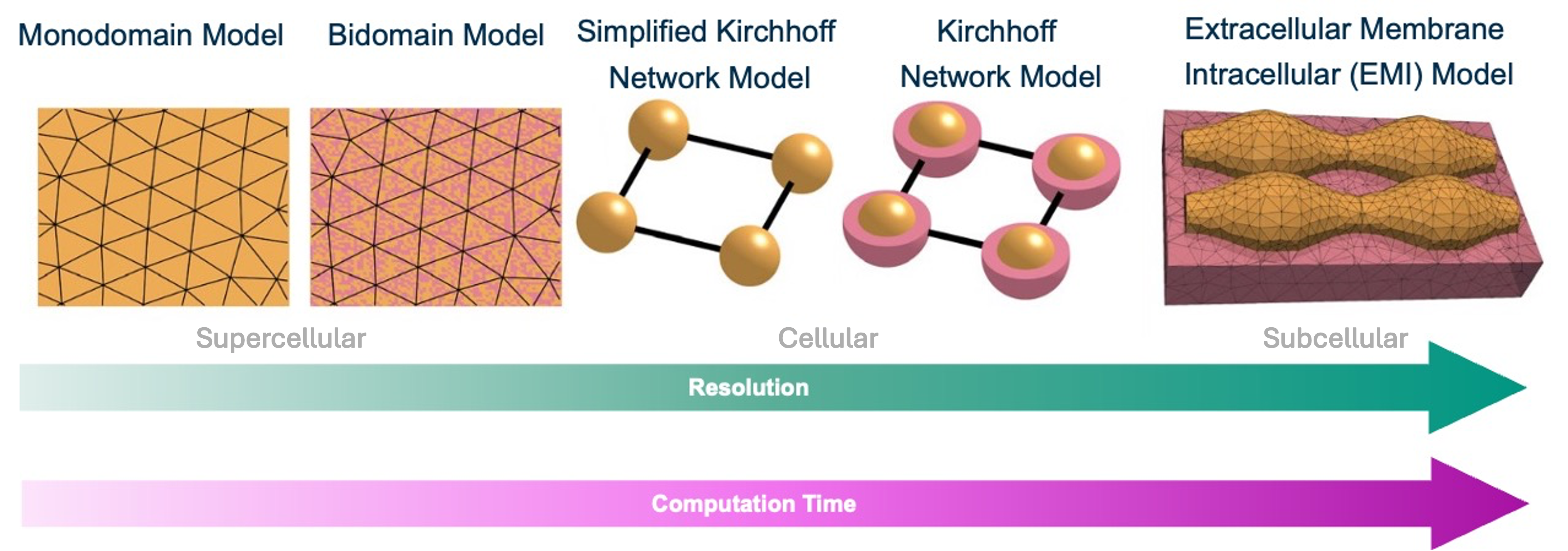
At one end of the spectrum are the mono- and bidomain models, in which the intra- and extracellular spaces are represented as continuous domains. These formulations allow computationally efficient simulations of electrical propagation and tissue-bath interactions. However, they rely on the homogenisation of cellular and tissue properties within each mesh element (comprising dozens to hundreds of biological cells), meaning that individual cells are not explicitly represented and cellular variability cannot be resolved on a cell-by-cell scale. The monodomain model further simplifies the bidomain formulation by assuming that intra- and extracellular conductivity tensors are proportional ² .

At the other end of the spectrum are EMI models, which explicitly represent each myocyte and the surrounding extracellular space. This allows modifications at cellular and sub-cellular scale, enabling highly detailed investigations of electrophysiological processes. However, such models require extremely fine meshes, which substantially increase computational cost ³ .

Lastly, the Kirchhoff network model (KNM) and its simplified variant SKNM, introduced by Jaeger et al. ^{4 5} , represent an intermediate modelling approach. In these models, each myocyte is represented as an individual node in an electrical network, whereas neighbouring cells are connected via resistive elements representing gap junctional coupling. This allows manipulation of cellular properties and intercellular coupling while avoiding the computational expense of resolving intra- and extracellular domains explicitly.

Consequently, the SKNM offers a useful compromise between high spatial resolution of the EMI models and the computational efficiency of the mono- and bidomain approaches.

Deriving the simplified Kirchhoff network model

By assuming each cell, and the corresponding extracellular space surrounding it, is a node on a computational grid, the currents between neighbouring nodes (cells) are calculated following Ohm's law:

\[I_\mathrm{i}^{j,k} = G_\mathrm{i}^{j,k} (\Phi_\mathrm{i}^{j} - \Phi_\mathrm{i}^{k}) I_\mathrm{e}^{j,k} = G_\mathrm{e}^{j,k} (\Phi_\mathrm{e}^{j} - \Phi_\mathrm{e}^{k}){,}\]

where \(G_\mathrm{i}^{j,k}\) and \(G_\mathrm{e}^{j,k}\) denote the conductances (in mS) connecting the intra- and extracellular spaces of the cells j and k. Furthermore, \(I_\mathrm{m}^{k}\), i.e. the total current flowing through the membrane of cell k, from intra- to extracellular space, is given by:

\[I_\mathrm{m}^k = A_\mathrm{m}^k(C_\mathrm{m} \frac{dV_\mathrm{m}^k}{dt} + I_\mathrm{ion}^k(s^k, V_\mathrm{m}^k)){,} \quad (1)\]

with state variables vector s. Applying Kirchhoff's current law to a cell, the current flowing out, i.e. \(I_\mathrm{m}^k\), must be equal to the sum of the currents flowing in from the \(N^k\) neighbouring cells:

\[I_\mathrm{m}^k = \sum \limits_{j\in N^k}I_\mathrm{i}^{j,k}{.} \quad (2)\]

Similarly, the application of Kirchhoff's current law to the extracellular space yields:

\[I_\mathrm{m}^k + \sum \limits_{j \in N^k}I_\mathrm{e}^{j,k} = 0{.}\]

Finally, rearranging Equation Equation 1 and substituting \(I_\mathrm{m}^{k}\) with Equation 2 yields the KNM system:

\[C_\mathrm{m} \frac{dV_\mathrm{m}^{k}}{dt} = \frac{1}{A_\mathrm{m}^{k}} \sum \limits_{{j}\in N^{k}}I_\mathrm{i}^{j,k} - I_\mathrm{ion}^{k}(s^{k}, V_\mathrm{m}^{k})\]

\[\sum \limits_{{j}\in N^{k}}I_\mathrm{i}^{j,k} + \sum \limits_{{j}\in N^{k}}I_\mathrm{e}^{j,k} = 0 \frac{ds^{k}}{dt}= F(s^{k}, V_\mathrm{m}^{k}){.}\]

\[\frac{ds^{k}}{dt}= F(s^{k}, V_\mathrm{m}^{k}){.}\]

The KNM can be simplified to the SKNM, analogous to the reduction of the bidomain to the monodomain model, by assuming that:

\[G_\mathrm{e}^{j,k} = \lambda G_\mathrm{i}^{j,k}{.} \quad (3)\]

Using Equation 3 and following the steps reported in ⁶ , the SKNM equations are obtained:

\[C_\mathrm{m} \frac{dV_\mathrm{m}^{k}}{dt} = \frac{1}{A_\mathrm{m}^{k}} \frac{\lambda}{\lambda + 1} \sum \limits_{{j}\in N^{k}}G_\mathrm{i}^{j,k}(V_\mathrm{m}^{j} - V_\mathrm{m}^{k}) - I_\mathrm{ion}^{k}(s^{k}, V_\mathrm{m}^{k})\]

\[\frac{ds^{k}}{dt}= F(s^{k}, V_\mathrm{m}^{k}){.}\]

Experiment setup

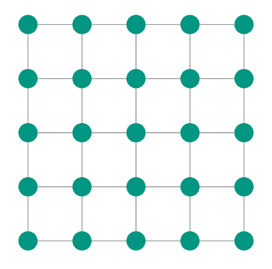
In this example, the finite element method (FEM) implementation of openCARP, which is typically used for mono- and bidomain simulations, is applied to a mesh composed solely of one-dimensional line elements (Figure 2). In this configuration, the monodomain solver of openCARP acts as a surrogate implementation of the SKNM. Thereby, each mesh node represents a single cell, while line elements connecting neighbouring nodes represent intercellular coupling. This setup enables node-wise adjustment of cellular properties through the adjustment file functionality of openCARP. Simultaneously, as each element connects exactly two cells, the properties of intercellular coupling can be modified by assigning different conductivities to individual elements through the gregions command. The setup shown here is isotropic with respect to both the node spacing in the mesh and the conductivities.

For comparison with a typical monodomain simulation workflow, see the Heterogeneities: region vs. gradients example. In that example, four differently parameterised ionic models are assigned to four regions of a square tissue patch, resulting in four homogeneous tissue areas. In contrast, the SKNM setup allows cell-wise heterogeneity through node-specific parameter adjustments.

Nevertheless, some differences remain compared to the original SKNM implementation, and the advantages and disadvantages of each approach can be debated. In openCARP, the mass matrix accounts for the reduced "volume" of boundary and corner nodes. As a result, the diffusion term at a corner node has the same magnitude as an interior node. In contrast, in the original SKNM formulation, the total current leaving a boundary node is strictly lower because it has fewer neighbours, unless the cross-sectional area \(\tilde{\mathrm{A}}\) is locally adjusted to reflect the boundary conditions. Consequently, the openCARP implementation effectively behaves as a normalised network, where the conductivity is scaled by the local connectivity to remain consistent with the underlying continuous cable partial differential equation (PDE) across the entire domain. Since other studies, such as Ricci et al. ⁷ , did not explicitly separate the contributions of intracellular conductivity and gap-junctional conductance to the overall intercellular coupling, we adopted the following formulation for the conductivities assigned to the line elements of the mesh:

\[g_\mathrm{i} = g_\mathrm{e} = 2 \frac{l_\mathrm{e}}{\tilde{A}R}{,}\]

where \(l_\mathrm{e}\) denotes the length of the element and coincides with the mesh resolution, \(R\) is the desired intercellular coupling resistance measured in \(\mathrm{M}\Omega\), and \(\tilde{\mathrm{A}}\) is the cross-sectional area of the line element. In this example, \(\tilde{\mathrm{A}}\) was set to \(1\,\mu\mathrm{m}^{2}\). The formulation follows from Ohm's law for a resistive conductor, where resistance depends on conductivity, length, and cross-sectional area.

To investigate the effects of heterogeneity, a square patch consisting of 25 nodes arranged on a \(5\times5\) grid was used. The nodes were equally spaced with a resolution of \(70\,\mathrm{\mu m}\), corresponding approximately to the size of a single sinoatrial node cell (SANC). The mesh used for this setup has been generated beforehand and is provided in the mesh directory of this example. It is directly loaded by the simulation script and therefore does not need to be generated during runtime. Each node was assigned a different parameter set of the extended Severi model ⁸ , sampled from the POM.

The POM approach is chosen for two reasons. The first is conceptual and essential. The extended Severi model describes rabbit SANCs, which are intrinsically self-exciting. If identical ionic models with identical initial conditions were assigned to every node in the tissue patch, all cells would exhibit identical spontaneous depolarisation. Consequently, no voltage differences would arise between neighbouring cells and the intercellular coupling current would vanish, making the simulation effectively equivalent to performing the same single-cell simulation at each node. The second reason is physiological. Ion channel turnover times range from hours to days and are influenced by genetic, environmental, and temporal factors ⁹ , ¹⁰ . This leads to pronounced variability in cellular electrophysiological properties that can be captured using a POMs approach. More information about POMs and the creation of a POM can be found in the Parallel single-cell example.

Run the simulation

To inspect all the options of this run.py script, execute it inside the example directory with the --help flag.

cd ${EXAMPLES}/04_sknm_tissue/01_sknm_san
python3 run.py --help

To run the simulation with the default settings, execute the run.py script without additional flags:

python3 run.py

This will execute a SKNM simulation of 500 ms using different SANC models sampled from the POM and store the results in a folder named with the current date and information about the simulation. The cells are virtually uncoupled because Rgap is set to 1e300 (i.e. very high) here by default. This means each cell depolarises independently and does not influence its neighbours. To assess the effects of coupling and execute multiple simulations with different coupling values, use the commented list in the main function.

In the terminal, you should see the command passed to openCARP, a few warnings (which in our case can be ignored, for example because no stimulus needs to be defined for SANC models), followed by mesh processing and ionic model initialisation.

To visualise the simulation results, Meshalyzer will open automatically in case it is installed and the simulation is executed with the --visualize flag.

python3 run.py --visualize

We now can appreciate a pattern similar to that in Figure 3: A \(5\times5\) grid of nodes solely connected via line elements. For each node and line element, the transmembrane voltage Vm is displayed. By pressing play button, the differently parametrised cell models start to depolarise automatically with different cycle lengths.

By clicking on Pick Vertex, selecting a node and then clicking on time series, you can view Vm values for the various nodes.

Note that the differently parametrised models were sampled from the file POM_parameters_baseline.csv. This file contains all the parameter values as well as all the state variables saved after running the corresponding single-cell simulation for 1,000,000.0 ms to reach a limit cycle. As a result, when the tissue simulation starts, the cells are already in different phases of the action potential. This can be seen from the different colours of the nodes, each representing to the Vm.

As a next step, we decrease the gap-junctional resistance to study the effect of electrical coupling between differently parametrised models. Here, we set Rgap to 1,000 \(\mathrm{M}\Omega\). Therefore, the simulation is executed with the --rgap flag.

python3 run.py --rgap 1000.0 --visualize

Meshalyzer should open and show a simulation similar to Figure 4. Compared to the virtually uncoupled case, this lower resistance allows currents to flow between neighbouring cells. When the simulation is re-run, the initially different cycle lengths start to influence each other, and the cells synchronise towards a common cycle length.

A comparison of the Time series of the various nodes with the virtually uncoupled simulation further emphasises the converging cycle length.

It is also possible to decrease the extracellular calcium concentration (Cao) or increase sympathetic stimulation by simulating different isoprenaline concentrations (Iso_cas). These changes affect the cycle length, which in turn can be observed by inspecting the Time series of the various nodes. An example with a clearly visible effect within the 500 ms simulation window can be obtained by setting --imp-par ANS=1.0,Cao=1.0. Note that the models used in this example are parametrised based on the baseline model, which was simulated for 1,000 s to reach a limit cycle. Consequently, the responses shown here illustrate the general behaviour, even though the results may differ slightly from simulations initialised with the corresponding modified conditions (these initial states are not included in this example; see POM_parameters_baseline.csv for the initial values of the baseline model after reaching a limit cycle length).

References

Recent questions tagged limpet, experiments, examples, tissue, sknm

References

Jæger, K. H. et al., Evaluating computational efforts and physiological resolution of mathematical models of cardiac tissue, Sci. Rep., vol. 14, p. 16954, 2024. DOI: 10.1038/s41598-024-67431-w↩︎
Jæger, K. H. and Tveito, A., The simplified Kirchhoff network model (SKNM): a cell-based reaction-diffusion model of excitable tissue, Sci. Rep., vol. 13, p. 16434, 2023. DOI: 10.1038/s41598-023-43444-9↩︎
Tveito, A. et al., Modeling Excitable Tissue: The EMI Frame-work, Simula SpringerBriefs on Computing, vol. 7. Cham: Springer International Publishing, 2021. DOI: 10.1007/978-3-030-61157-6↩︎
Jæger, K. H. and Tveito, A., Efficient, cell-based simulations of cardiac electrophysiology; The Kirchhoff Network Model (KNM), npj. Syst. Biol. Appl., vol. 9, p. 25, 2023. DOI: 10.1038/s41540-023-00288-3↩︎
Ricci, E. et al., Sinoatrial node heterogeneity and fibroblasts increase atrial driving capability in a two-dimensional human computational model, Frontiers in Physiology, vol. 15, 2024. DOI: 10.3389/fphys.2024.1408626↩︎
Linder, M. et al., Sympathetic stimulation can compensate for hypocalcaemia-induced bradycardia in human and rabbit sinoatrial node cells, The Journal of Physiology, 2025. DOI: 10.1113/jp287557↩︎
Lawson, B. A. J. et al., Unlocking data sets by calibrating populations of models to data density: A study in atrial electrophysiology, Science Advances, vol. 4, p. e1701676, 2018. DOI: 10.1126/sciadv.1701676↩︎
Maltsev, V. A. et al., Molecular identity of the late sodium current in adult dog cardiomyocytes identified by Nav 1.5 antisense inhibition, American Journal of Physiology-Heart and Circulatory Physiology, vol. 295, pp. H667-H676, 2008. DOI: 10.1152/ajpheart.00111.2008↩︎