EMI stimulation modes
See code in GitLab.
Author: Tobias Gerach tobias.gerach@kit.edu
To run the experiments of this example:
cd ${EXAMPLES}/07_EMI/01_stimulationEMI stimulation modes
Cardiac tissue can be excited by establishing an extracellular electric field, by injecting or withdrawing current through electrodes, or by delivering current directly across the cell membrane. In bidomain or monodomain models, these reduce to two broad families (voltage-domain and current-domain), because the intracellular and extracellular domains are coupled implicitly through the homogenised membrane conductance. The EMI model resolves all three domains explicitly — intracellular \(\Omega_\mathrm{i}\), extracellular \(\Omega_\mathrm{e}\), and the membrane interface \(\Gamma_\mathrm{m}\) — and therefore supports a richer set of stimulus circuit types.
This example walks through eight stimulus protocols, grouped by the domain in which they act:
- Extracellular (\(\Omega_\mathrm{e}\)) — six protocols driven through electrodes in the extracellular domain, as either a voltage or a current source, closed- or open-loop, closed by a Dirichlet ground or — for a pure Neumann problem — by nullspace stabilisation. All six are calibrated to impose the same mean field of 2 V/cm across the electrode gap and therefore yield almost identical solutions. Their agreement is a self-consistency check on the circuit types, not a parameter study: what differs is only the wiring — how the reference potential is fixed and whether the source stays connected after the pulse.
- Intracellular (\(\Omega_\mathrm{i}\)) — a sharp microelectrode that injects
current at a single site inside the cytoplasm of one cell (
INTRA_I). This is the computational analogue of a current-clamp impalement or whole-cell patch, the standard way single cardiomyocytes are paced in the laboratory. EMI can represent it faithfully because it resolves the cell interior; homogenised models cannot. - Transmembrane (\(\Gamma_\mathrm{m}\)) — current delivered directly across
the membrane (
MEMBRANE_I). This is the stimulus abstraction inherited from monodomain and bidomain models; no single physical device sits behind it, but it is the simplest and most robust way to depolarise the membrane when the goal is merely to initiate an action potential rather than to reproduce an experimental setup.
All stimuli use a 2 ms pulse, and an action potential initiated in any cell
propagates along the whole chain through the gap junctions (fig-emi-stim-mesh).
The voltage and current circuit types can equally clamp or inject in
\(\Omega_\mathrm{i}\) directly (crct.type 10/11 voltage clamp,
crct.type = 4 current); the intracellular voltage clamp is left out here because
its purpose is to measure current under a controlled membrane potential, not to
initiate propagation.
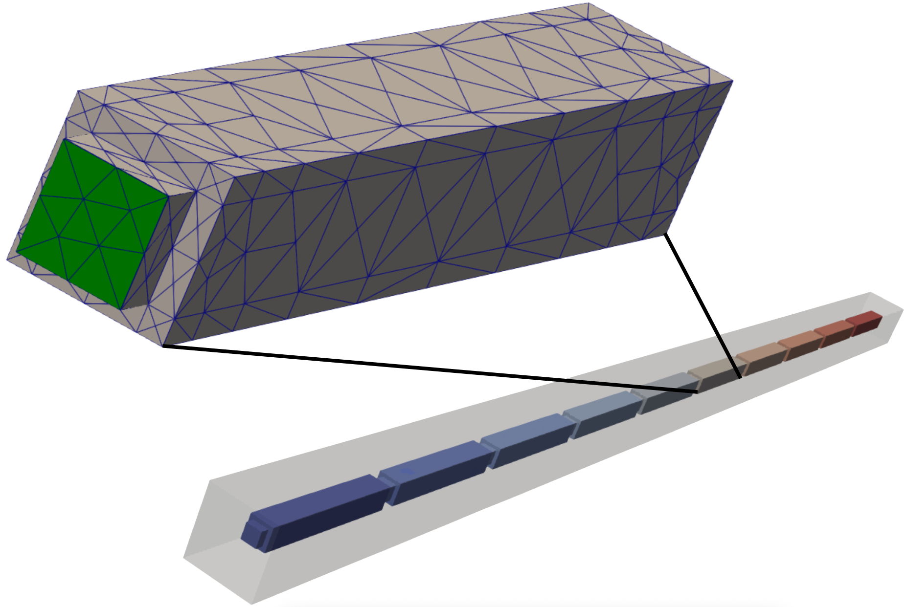
Computational mesh
All experiments share a single tetrahedral mesh, mesh/chain_reindex
(fig-emi-stim-mesh). Ten cardiomyocytes are placed end to end along
\(x\), each carrying its own intracellular tag, and are embedded in a common
extracellular domain (a single extracellular tag) that extends 15 µm beyond the
cells on every side. The full block measures 1130 × 45 × 45 µm`^3`. Adjacent cells
are coupled across their intercalated discs \(\Gamma_\mathrm{g}\) by gap
junctions (Plonsey model, \(R_\mathrm{m} = 0.0045\,\mathrm{k\Omega\,cm^2}\))
so that an action potential initiated in any cell propagates along the entire
chain.
Electrode setup
Three electrodes are placed on the chain mesh at run time using its bounding box:
- A — left end-plate spanning the full y/z cross-section of the extracellular domain; acts as the anode or current-injection site in most modes.
- B — right end-plate spanning the full y/z cross-section; acts as the cathode or ground.
- C — small patch on the top extracellular surface at the x-centre of the chain; used as a potential reference in balanced configurations.

The electrode geometry is derived by calling _generate_electrodes at the start
of each run. The A–B gap for this mesh is 1115 µm (electrode inner faces).
Overview
| Protocol | Domain | crct.type |
Reference | Physical analogue |
|---|---|---|---|---|
EXTRA_V |
\(\Omega_\mathrm{e}\) | 2 (+ 3) | ground at B | voltage-source field stimulation |
EXTRA_V_BAL |
\(\Omega_\mathrm{e}\) | 2 + 2 (+ 3) | centre ground at C | symmetric voltage field |
EXTRA_V_OL |
\(\Omega_\mathrm{e}\) | 5 (+ 3) | ground at B; A floats after pulse | voltage stimulation, electrode released |
EXTRA_I |
\(\Omega_\mathrm{e}\) | 1 (+ 3) | ground at B | current-source field stimulation |
EXTRA_I_BAL |
\(\Omega_\mathrm{e}\) | 1 + 1 | none — nullspace | charge-balanced bipolar current |
EXTRA_I_BAL_GND |
\(\Omega_\mathrm{e}\) | 1 + 1 (+ 3) | centre ground at C | bipolar current with drain |
INTRA_I |
\(\Omega_\mathrm{i}\) | 4 | none — nullspace | sharp microelectrode / patch current clamp |
MEMBRANE_I |
\(\Gamma_\mathrm{m}\) | 0 | none — nullspace | direct transmembrane injection (model abstraction) |
Extracellular voltage stimulation
Extracellular voltage stimulation enforces a prescribed time course on \(\phi_\mathrm{e}\) at an electrode surface, i.e. it imposes a Dirichlet boundary condition in \(\Omega_\mathrm{e}\):
\[\phi_\mathrm{e}(\mathbf{x}, t) = f(t) \quad \forall\, \mathbf{x} \in \Gamma_\mathrm{D}.\]
At least one such Dirichlet condition must be present for the elliptic problem to
have a unique solution. In openCARP the closed-loop Dirichlet type is
crct.type = 2; the open-loop variant (electrode floats after the pulse) is
crct.type = 5; a pure ground (zero potential) is crct.type = 3.
The applied potential is set so that the mean field across the A–B gap matches the default 2 V/cm: \(V_{AB} = E \cdot d_{AB} = 2\,\mathrm{V/cm} \times 1115\,\mu\mathrm{m} = 223\,\mathrm{mV}\).
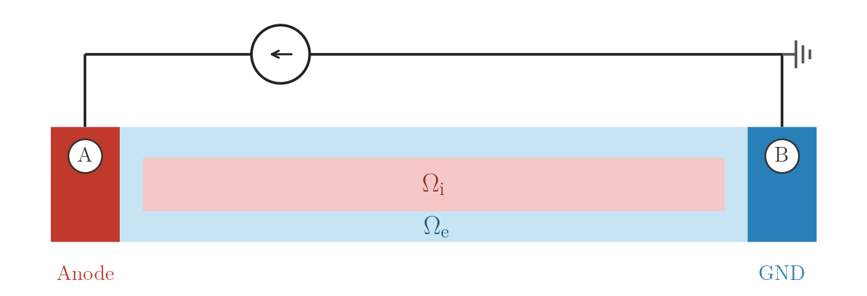
EXTRA_V — closed-loop extracellular voltage clamp
Electrode A is clamped to \(V_A = E \cdot d_{AB}\) for the 2 ms pulse; electrode B is grounded at zero potential throughout. After the pulse ends, A is driven back to 0 mV (closed-loop: the voltage source remains connected).
Because positive \(\phi_\mathrm{e}\) at A raises the extracellular potential locally it hyperpolarises the adjacent membrane (anodal effect), while the grounded B acts as a cathode and depolarises tissue in its vicinity.
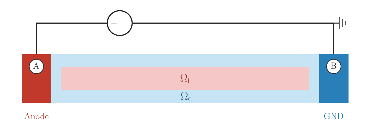
EXTRA_V: closed-loop voltage source at A, ground at B.numstim = 2
# electrode A
stim[0].crct.type = 2 # closed-loop extracellular voltage clamp
stim[0].pulse.strength = 223.0 # V_A = E·d_AB (mV); d_AB = 1115 µm
# electrode B
stim[1].crct.type = 3 # ground./run.py --stimulus EXTRA_V --visualizeEXTRA_V_BAL — balanced extracellular voltage
A is clamped to \(+S\), B mirrors A with opposite polarity via crct.balance,
so the total potential drop is \(V_{AB} = 2S = E \cdot d_{AB}\). Electrode C
is grounded at the extracellular mid-point, anchoring the zero-potential isoline to the
centre of the chain and producing a symmetric extracellular field about C.
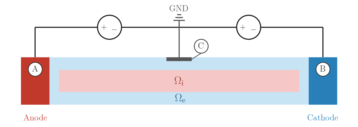
EXTRA_V_BAL: symmetric voltage sources with centre GND at C.numstim = 3
# electrode A
stim[0].crct.type = 2 # closed-loop voltage clamp
stim[0].pulse.strength = 111.5 # +½·E·d_AB (mV)
# electrode B
stim[1].crct.type = 2 # mirrored source, linked to stim[0] by crct.balance
stim[1].crct.balance = 0 # index of the reference electrode
# electrode C (top extracellular surface, x-centre)
stim[2].crct.type = 3 # ground — fixes the potential reference./run.py --stimulus EXTRA_V_BAL --visualizeEXTRA_V_OL — open-loop extracellular voltage
Same applied potential as EXTRA_V, but at \(t = 2\,\mathrm{ms}\) electrode
A is disconnected from the source (crct.type = 5) rather than being driven
back to 0 mV. After the pulse the electrode floats and the local potential evolves
freely with the extracellular field. Electrode B remains grounded throughout.
Compared to EXTRA_V, the floating A node no longer acts as a second ground after
\(t_\mathrm{off}\), which alters the post-stimulus redistribution of
\(\phi_\mathrm{e}\) and can affect repolarisation dynamics.
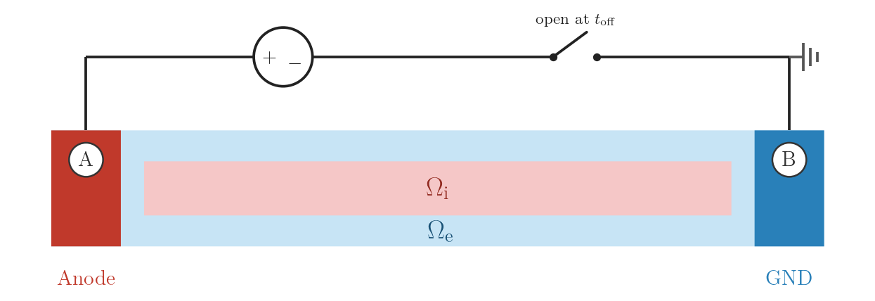
EXTRA_V_OL: voltage source at A with open switch at
\(t_\mathrm{off}\), ground at B.numstim = 2
# electrode A
stim[0].crct.type = 5 # open-loop voltage (electrode floats at t_off)
stim[0].pulse.strength = 223.0 # same magnitude as EXTRA_V (mV)
# electrode B
stim[1].crct.type = 3 # ground./run.py --stimulus EXTRA_V_OL --visualizeExtracellular current stimulation
Current stimulation injects or withdraws charge through volumetric sources placed in \(\Omega_\mathrm{e}\). The FEM assembles these as contributions to the right-hand side without modifying the system matrix. Injecting current at A raises \(\phi_\mathrm{e}\) locally (hyperpolarisation, anodal effect); withdrawing current at a grounded B lowers \(\phi_\mathrm{e}\) there (depolarisation, cathodal effect).
When no Dirichlet ground is present the extracellular problem is a pure Neumann problem: the solution is unique only up to an additive constant. openCARP detects this and attaches a nullspace projection to the solver, enforcing the constraint
\[\int_{\Omega_\mathrm{e}} \phi_\mathrm{e}\,\mathrm{d}\Omega = 0.\]
The stimulus strength for all EXTRA_I modes is set via a 1-D parallel-conductor
estimate so that the mean field across the A–B gap matches 2 V/cm:
\(I = E(\sigma_\mathrm{e}\,A_\mathrm{e} + \sigma_\mathrm{i}\,A_\mathrm{i}) \approx 0.74\,\mu\mathrm{A}\).
EXTRA_I — extracellular current injection
Current \(I_A\) is injected at electrode A (crct.total_current = 1 selects
mesh-independent total-current mode) and collected at the grounded electrode B.
EXTRA_I: current source at A, ground at B.numstim = 2
# electrode A
stim[0].crct.type = 1 # extracellular current injection
stim[0].crct.total_current = 1 # total-current mode (mesh-independent)
stim[0].pulse.strength = 0.738 # I_A (µA)
# electrode B
stim[1].crct.type = 3 # ground (collects the injected current)./run.py --stimulus EXTRA_I --visualizeEXTRA_I_BAL — balanced bipolar current, no ground
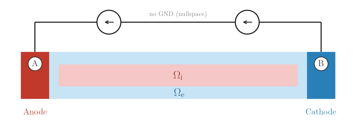
A injects \(+I\), B withdraws \(-I\) (crct.balance). Net current
is zero, satisfying the compatibility condition for the pure Neumann problem.
openCARP resolves the additive constant via nullspace stabilisation.
EXTRA_I_BAL: bipolar current sources, no ground
(nullspace stabilisation).numstim = 2 # no ground electrode
# electrode A
stim[0].crct.type = 1
stim[0].crct.total_current = 1
stim[0].pulse.strength = 0.738 # I_A (µA)
# electrode B
stim[1].crct.type = 1 # current withdrawal
stim[1].crct.balance = 0 # mirrors strength of stim[0] with opposite sign./run.py --stimulus EXTRA_I_BAL --visualizeEXTRA_I_BAL_GND — balanced bipolar current with ground
Same as EXTRA_I_BAL with an additional Dirichlet ground at C. The ground
uniquely determines the potential without nullspace stabilisation. Any residual
current imbalance between A and B drains through C.

EXTRA_I_BAL_GND: bipolar current sources with centre GND at C.numstim = 3
# electrode A
stim[0].crct.type = 1
stim[0].crct.total_current = 1
stim[0].pulse.strength = 0.738
# electrode B
stim[1].crct.type = 1
stim[1].crct.balance = 0
# electrode C (top extracellular surface, x-centre)
stim[2].crct.type = 3 # ground — uniquely determines the solution./run.py --stimulus EXTRA_I_BAL_GND --visualizeIntracellular current stimulation
Intracellular current stimulation injects current directly into the cytoplasm
\(\Omega_\mathrm{i}\) of a single cell (crct.type = 4). Because EMI resolves
the cell interior, the electrode can be a small sphere placed at one point inside the
cell — a faithful model of a sharp microelectrode impaling the cytoplasm, or of a
whole-cell patch pipette. This is how single cardiomyocytes are most commonly paced
experimentally and, unlike the transmembrane abstraction below, it corresponds to a
real device.
INTRA_I — intracellular current injection (sharp microelectrode)
A 0.005 µA, 2 ms current is injected at a single intracellular site near the centre
of the leftmost cell, using a sphere electrode (elec.geom_type = 1) in
total-current mode. The stimulated cell depolarises and the action potential
propagates through the gap junctions to the rest of the chain — the same outcome as
MEMBRANE_I, but delivered through the intracellular domain rather than across the
membrane.

INTRA_I: point current source inside the leftmost
cell; no external electrodes.numstim = 1 # single intracellular electrode (sphere, leftmost cell)
# sharp microelectrode in the cytoplasm of cell 1
stim[0].crct.type = 4 # intracellular current injection
stim[0].crct.total_current = 1 # total-current mode (mesh-independent)
stim[0].pulse.strength = 0.005 # injected current (µA)
stim[0].elec.geom_type = 1 # sphere electrode (point impalement)./run.py --stimulus INTRA_I --visualizeTransmembrane current stimulation
Transmembrane stimulation delivers current directly at the membrane interface
\(\Gamma_\mathrm{m}\) (crct.type = 0). Unlike the extracellular and
intracellular electrodes it does not correspond to a specific physical device: it is
the stimulus abstraction inherited from monodomain and bidomain models, where the
membrane current is the natural forcing term. That makes it the simplest and most
robust way to initiate an action potential when the experimental setup is not the
point and one only needs the membrane to depolarise. The stimulated cell
depolarises directly and the action potential propagates through the gap junctions
to all ten cells.
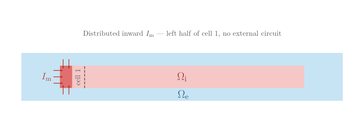
MEMBRANE_I — direct transmembrane current injection
A 150 µA/cm², 2 ms inward current is applied to the membrane faces covering the left half (in x) of the leftmost myocyte. openCARP restricts the electrode to the membrane interface automatically.
Because there is no extracellular field the action potential propagates right-ward uniformly through gap junctions, activating all ten cells.
MEMBRANE_I: distributed inward transmembrane current
on the left half of cell 1; no external electrodes.numstim = 1 # single membrane-patch electrode (left half of cell 1)
# membrane patch on the left half of cell 1
stim[0].crct.type = 0 # transmembrane current injection
stim[0].pulse.strength = 150 # I_m (µA/cm²)./run.py --stimulus MEMBRANE_I --visualizeVisualisation
With --visualize, meshalyzer opens the transmembrane voltage vm.igb on
the membrane sub-mesh <basename>_m with the pre-configured view in
stimulation.mshz. The extracellular potential phie.igb is written on the
volumetric sub-mesh <basename>_e and can be opened in a second window to
inspect \(\phi_\mathrm{e}\). Both fields are dumped for every stimulus
protocol, so the same procedure applies to all modes.
To plot the data in ParaView instead, first merge each field with its sub-mesh
using meshtool collect, which writes a single time-resolved mesh file:
# extracellular potential (nodal data on the _e sub-mesh)
meshtool collect -imsh=chain_reindex_e -omsh=phie -nod=phie.igb -inc=10

# transmembrane voltage (element data on the _m sub-mesh)
meshtool collect -imsh=chain_reindex_m -omsh=vm -ele=vm.igb -inc=10
Here -imsh is the sub-mesh basename, -omsh the output basename, -nod
/ -ele attach the IGB as nodal or element data respectively, and -inc
sets the time-step increment (every 10th frame here). Run meshtool collect
without arguments for the full option list.
INTRA_I protocol, rendered in ParaView. Top:
extracellular potential \(\phi_\mathrm{e}\); bottom: transmembrane
potential \(V_\mathrm{m}\). Current injected at a single intracellular
site in the leftmost cell depolarises it, and the action potential propagates
along the chain through the gap junctions.Usage
cd examples/07_EMI/01_stimulation

# closed-loop extracellular voltage clamp (default)
./run.py --stimulus EXTRA_V --visualize

# intracellular sharp-microelectrode injection in the leftmost cell
./run.py --stimulus INTRA_I --visualize

# transmembrane stimulation, AP propagates through all ten cells
./run.py --stimulus MEMBRANE_I --visualize

# override stimulus strength (µA/cm² for MEMBRANE_I, total µA for INTRA_I)
./run.py --stimulus MEMBRANE_I --strength 200 --visualize
Recent questions tagged EMI, carputils, stimulation
There are tagged with EMI, carputils, stimulation.
Here we display the 5 most recent questions. You can click on each tag to show all questions for this tag.
You can also ask a new question.