Lead field ECG
See code in GitLab.
Author: Julian Mierisch julian.mierisch@kit.edu, Tobias Gerach tobias.gerach@kit.edu
Overview
This example demonstrates the practical application of the lead field method for reconstructing electrocardiograms (ECGs) from monodomain or reaction-eikonal simulations. Unlike the standard bidomain approach, which solves for extracellular potentials at every time step, the lead field method splits the problem into two stages: a static computation of the volume conductor's sensitivity, followed by a dynamic projection of cardiac sources. We will use a simplified geometric model in this example. For a theoretical breakdown of the lead field math, refer to the related section of the openCARP manual.
To run this example, change directories as follows:
cd ${EXAMPLES}/02_EP_tissue/09_leadfieldObjectives
After having worked through this example, you should be able to:
- Understand the mathematical foundation of the lead field method, including how it decouples the spatial and temporal components of ECG reconstruction.
- Compute the lead field vectors for a given geometry and electrode configuration using openCARP's post-processing capabilities.
- Explore the modularity of the lead field approach, including how to reuse pre-computed sensitivity maps and voltage data for rapid ECG calculations.
Setup
The experiment utilizes a controlled simplified geometry to validate the method without anatomical complexity:
- Geometry: Two central cubic blocks of active cardiac tissue (the "heart") are stacked vertically within a larger, passive conductive torso block.
- Electrodes: A complete 12-lead ECG configuration is used, with electrodes placed strategically on the surface of the torso block to capture both limb and precordial signals.
- Stimulation: The simulation initiates two distinct planar wavefronts: first at the back-left-top corner of the upper block (propagating downward), followed by the front-right-bottom corner of the lower block after a set delay (propagating upward). The two waves converge toward the passive tissue gap between the blocks.
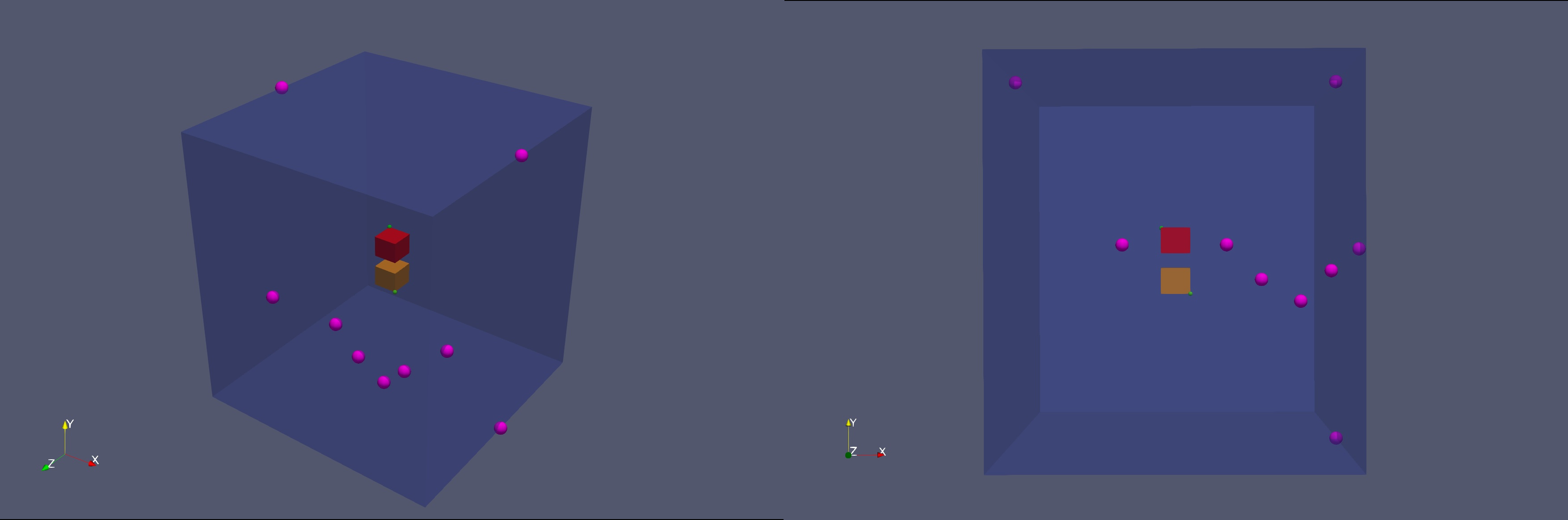
Angled and frontal view of the mesh with stimuli and electrode positions. This setup ensures a predictable voltage gradient, resulting in a clear deflection in the computed ECG.
Input Parameters
The following input parameters are exposed to steer the experiment:
--bidomain INT
                    Choose simulation method (default: 0) (options: monodomain=0, bidomain=1, pseudobidomain=2).

--resolution FLOAT
                    Choose mesh resolution in [um] (default: 250 um).

--lf_vmfile STRING
                    Path to the transmembrane voltage data file (default: '').

--lf_dir STRING
                    Path to the directory in which the lead field data resides (default: '').

--lf_config INT
                    Choose lead configuration (default: 12) (options: 1, 3, 5, 12).

--ecg_timedt FLOAT
                    ECG time resolution in [ms] (default: 1 ms) (cannot be smaller than the time resolution of the simulation).

--post_processing_opts INT
                    Choose which postprocessing option to run (default: 64).

--electrodes STRING
                    Path to the directory with the electrode positions (default: 'electrodes').
Expected Results
Upon successful completion of the example, the output defines both the spatial sensitivity of the electrodes and the resulting temporal signals per lead. The lead field vectors are generated for each lead and saved in IGB format; visualizing these files reveals the sensitivity distribution across the cardiac mesh. By combining these spatial weights with the simulated transmembrane voltages, we compute the final ECG traces, which are exported as .dat files.
Experiment
In this example, we execute an end-to-end pipeline: we simulate two converging electrical wavefronts in the heart tissue blocks (monodomain), and in the same run, construct the lead field vectors and compute the ECG traces.
Note: While this example runs the full pipeline, advanced users can use the '--lf_dir' flag and the '--lf_vmfile' flag to run these steps modularly (e.g., skipping the simulation to re-calculate ECGs for existing vm.igb files).
Mandatory Parameters
To activate the lead field features during the run, specific parameters must be set (which is the case using the default parameters):
--lf_config: Defines the lead layout (e.g., 3-lead, 5-lead, 12-lead). This is passed to the underlyingcarputilshelper script to set up the electrodes.--ecg_timedt: Defines the temporal resolution of the ECG. This can be coarser than the simulation timestep (e.g., 1ms) to save storage.--post_processing_opts: Crucial. This bit-flag explicitly activates the lead field post-processing module in openCARP (e.g., 64 for lead field computation).--electrodes: Path to the directory containing electrode coordinates (e.g.,LA.vtx,LL.vtx, ...).
Running the Simulation
To run this example, execute the following command to start the full pipeline. We set the resolution to 250 \(\mu m\) (using the parameter's default value) and enable the standard 12-lead configuration.
python run.py --lf_config 12 --electrodes electrodesAfter the program finishes, check the POSTPROC_DIR. It will contain:
LF_*.igb: The spatial lead field vectors for each lead.ECG_*.dat: The computed temporal voltage traces.
Understanding the Example
Step 1: Visualizing Sensitivity
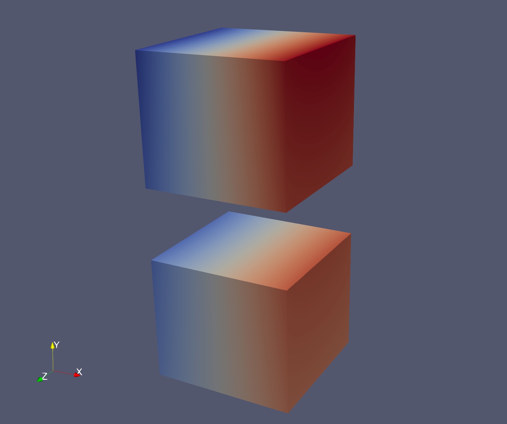
Before analyzing the signals, we inspect the sensitivity maps to verify that our virtual electrodes are correctly oriented. Load the LF_*.igb files in Meshalyzer or Paraview (see the examples in the visualization section to learn how to do this).
Step 2: Validating the ECG
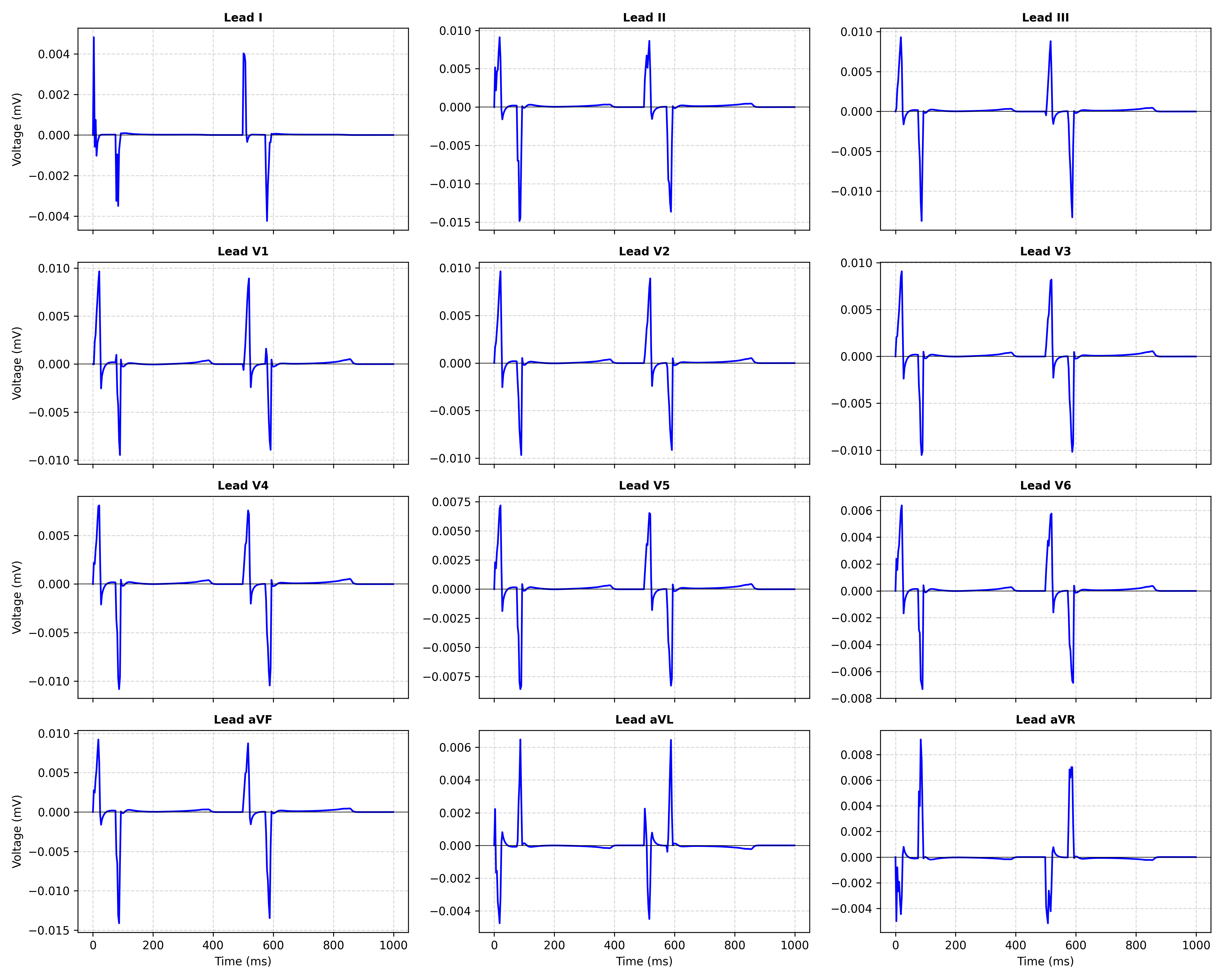
Next, we plot the ECG_*.dat files to verify that the simulation correctly captured the physics of our two converging wavefronts. Each lead shows two complexes per cycle (the S1 and S2 events, 75 ms apart), repeated twice over the 1000 ms simulation.
Lead I
- Lead I shows small but non-zero biphasic deflections (~±0.004 mV).
- Unlike a symmetric top-to-bottom setup, our stimuli are placed at opposite diagonal corners (back-left-top and front-right-bottom), introducing a lateral component that makes Lead I non-zero.
Leads II, III, and aVF
- These are the largest amplitude leads (II and aVF reach ~±0.015 mV, III ~±0.010 mV).
- Each complex shows two sequential biphasic deflections: one from S1 (upper block) and one from S2 (lower block, 75 ms later), with opposite polarity since the two wavefronts travel in opposite vertical directions.
Leads aVR and aVL
- These leads show moderate amplitude (aVR ~±0.008 mV, aVL ~±0.006 mV) and biphasic patterns.
- The polarity of each sub-deflection is opposite to that seen in Leads II, III, and aVF, consistent with the superior electrode positions viewing the same wavefronts from the opposite direction.
Precordial Leads (V1-V6)
- All precordial leads show biphasic complexes (~±0.010 mV for V1/V2, decreasing toward V6).
- S1 propagates from the back-left corner toward the front-right, producing the first sub-deflection. S2 propagates from the front-right corner toward the back-left, producing a second sub-deflection of opposite sign.
Advanced: Modular Workflows
One of the major advantages of the lead field method is its modularity. You do not always need to run the full pipeline. You can reuse expensive simulation results or pre-computed sensitivity maps to save time.
Note: A runtime comparison for realistic geometries will be added at a later point, quantifying the computation time saved by using the lead field method across different geometries.
The script automatically detects which stages to skip based on which flags you provide: pass --lf_vmfile to skip the cardiac simulation, pass --lf_dir to skip lead field construction, or pass both to bypass everything except the final ECG projection.
Scenario 1: Skipping the Cardiac Simulation (Post-Processing Only)
If you have already run a long excitation propagation simulation and saved the transmembrane voltage (\(V_m\)), you can compute the ECG, or re-compute it with a different temporal resolution, without re-running the excitation propagation simulation.
Required Input:
--lf_vmfile: Path to your existing voltage data (e.g.,vm.igb).
Command:
python run.py --lf_vmfile test_vm.igb --lf_config 12 --electrodes electrodesThe program skips the cardiac simulation. It immediately calculates the lead field matrices and projects the provided vm.igb data onto them to compute the ECG.
Scenario 2: Using Pre-Computed Lead Fields
If you want to run multiple different simulations (e.g., different pacing sites or conductivity values) on the same geometry, you can reuse the lead fields. If the electrode positions, tissue shape and conductive properties haven't changed, the lead field matrices are identical. You can point the pipeline to a directory containing existing lead field files to skip the construction step.
| Simulation Change | Reusable? | Note |
|---|---|---|
| Pacing / stimulus location (S1, S2) | YES | Changes only the source \(V_m\). |
| Stimulus timing / BCL | YES | Changes only the source \(V_m\). |
| Ionic model / cell parameters | MAYBE | In isolation changes only \(V_m\). If conduction velocity is re-tuned (e.g. tuneCV) after a model change, myocardial conductivity can change and therefore \(Z_L\). Exact reuse only if \(\sigma\) is deliberately held fixed. |
| Intracellular conductivity \(\sigma_i\) | NO (see below) | Enters the bulk conductivity \(\sigma_i+\sigma_e\) of the elliptic stiffness (sum_cond). |
| Extracellular conductivity \(\sigma_e\) | NO | Enters the bulk conductivity \(\sigma_i+\sigma_e\) of the elliptic stiffness (sum_cond). |
| Fiber orientation | NO | Sets the anisotropy of the bulk tensor. |
| Torso geometry | NO | Fundamentally alters the physical domain of the stiffness matrix. |
| Electrode placement | NO | Changes the mathematical definition of the lead and its associated sensitivity vector. |
Note: The table reflects what is theoretically correct; in practice there is some leeway, since the magnitude of each effect varies. \(Z_L\) is dominated by the outer volume conductor (torso/bath geometry, their conductivity, and the electrodes); the heart is a comparatively small volume, so a conductivity change confined to it often perturbs \(Z_L\) only weakly. In an attempt to quantify this, we made reduced the conductivity of the front half of the upper cardiac block by 10x (representing fibrotic tissue) and compared the ECG from a freshly recomputed \(Z_L\) against one that reused the control/healthy \(Z_L\). The transmembrane voltage \(V_m\) is identical in both, so the difference isolates the lead field error. Reusing the stale lead field leads to a ~5% mean RMS error per lead (up to ~10% in V1; limb leads ~2%). For comparison, the change in cardiac tissue conductivity itself changed the ECG by ~36% mean (up to ~68% in V1) relative to control/healthy. The conductivity change is thus carried almost entirely by \(V_m\); the lead field is less sensitive, and the largest reuse errors appear in the precordial leads (V1-V6) closest to the modified tissue. This robustness does not extend to changes in the torso geometry, bath conductivity, or electrode positions, which reshape \(Z_L\) more significantly.
Required Input:
--lf_dir: Path to the directory containing pre-computedLF_*.igbfiles.
Command:
python run.py --lf_dir test_leadfields --lf_config 12 --electrodes electrodesThe script runs the cardiac simulation, but it skips construction of the lead field vectors. It simply loads the LF_*.igb files from the folder and calculates the ECG on the fly.
Scenario 3: Turbo Mode
If you have pre-computed lead fields and pre-computed voltage data, you can use the "Turbo Mode". This can be used for rapid debugging of post-processing scripts or testing different ECG temporal resolutions (--ecg_timedt) without solving any differential equations.
By providing both the lead field directory and the voltage file, you bypass nearly the entire pipeline, performing only the final projection.
Required Input:
--lf_dir: Uses existing lead field sensitivity maps.--lf_vmfile: Uses existing transmembrane voltage data.
Command:
python run.py --lf_dir test_leadfields --lf_vmfile test_vm.igb --lf_config 12 --electrodes electrodesThe script skips both the tissue simulation and the lead field construction. It immediately loads both sets of data and performs the matrix-based dot product to output the ECG traces.
Carputils Lead Field Helper Script
The leadfield.py script serves as the wiring center for ECG simulations within the openCARP framework. Its primary purpose is to automate the mapping of virtual electrodes to specific simulation parameters, ensuring that the mathematical definitions of standard ECG leads (e.g., Wilson Central Terminal or augmented limb leads) are applied accurately.
The module translates high-level configuration choices (e.g., "12-lead ECG") into the detailed command-line arguments required by the openCARP solver. It manages three critical tasks:
- Electrode Mapping: It associates specific vertex files (
.vtx) with stimulation indices. - Weighting Logic: It implements the specific current injection patterns (sources and sinks) required to calculate differential potentials, such as the Wilson Central Terminal.
- Parameter Generation: It formats these configurations into the stimulus syntax expected by openCARP.
To utilize this module in an experiment script (like run.py), call the leadfield_setup() function. This function requires the desired configuration index and the path to the directory containing your electrode vertex files:
# Example: Setup for a standard 12-lead ECG
# Parameters: (config_index, electrodes_directory)
lf_stim_cmds, lf_elec_cmds, lf_run_opts = leadfield_setup(12, 'path/to/electrodes/')
The function returns three lists of command-line parameters (lf_stim_cmds, lf_elec_cmds, and lf_run_opts) that must all be appended to your main carp_cmd list.
The module currently supports the following standard layouts:
| Configuration Index | Leads Included | Required Electrodes |
|---|---|---|
| 1 | Bipolar (Single Lead) | Positive, Negative |
| 3 | Standard Limb (I, II, III) | RA, LA, LL |
| 5 | Limb + V1 (+ aVR, aVL, aVF + ground) | RA, LA, LL, V1 |
| 12 | Full Clinical 12-Lead | RA, LA, LL, V1-V6 |
The script is designed to be modular, allowing users to define custom lead configurations by following these steps:
- Update the config_map: In
leadfield_setup(), add a new index to the dictionary and list the required electrode names. - Implement Build Functions: Create a new pair of functions (e.g.,
build_custom_stims()andbuild_custom_electrodes()) to define the electrical poles and weights for your new leads. - Update the Dispatcher: Add a new case to the
match num_lead_electrodesblock inconfigure_leadfield()to trigger your custom build functions.
This abstraction allows openCARP to remain focused on the physics of the volume conductor, while this carputils layer handles the diverse requirements of various clinical and experimental lead layouts.
Recent questions tagged experiments, examples, tissue, ecg, lead field
There are tagged with experiments, examples, tissue, ecg, lead field.
Here we display the 5 most recent questions. You can click on each tag to show all questions for this tag.
You can also ask a new question.