Multiple Ionic Models On A Realistic Geometry
See code in GitLab.
Author: Joshua Steyer joshua.steyer@kit.edu
To run the experiments of this example:
cd ${EXAMPLES}/07_EMI/02_multi_ionicsMultiple ionic models on a realistic geometry
One advantage of the Extracellular-Membrane-Intracellular (EMI) model is that cardiac cells are represented explicitly within the computational domain, which enables studies with microstructurally varying electrophysiological properties. We here demonstrate this by modelling excitation wave propagation around a scar.
Mesh
The mesh is not part of the experiments repository because of its size.
Download it from Zenodo and unpack it into the example directory:
cd ${EXAMPLES}/07_EMI/02_multi_ionics
curl -L -o C5_mesh.tar.gz \
     https://zenodo.org/api/records/22047048/files/C5_mesh.tar.gz/content
tar xzf C5_mesh.tar.gz
This yields the binary mesh C5.bpts/C5.belem together with the tag
lists C5.intra and C5.extra (105 MB unpacked). The mesh is archived
at doi:10.5281/zenodo.22047047.
Setup
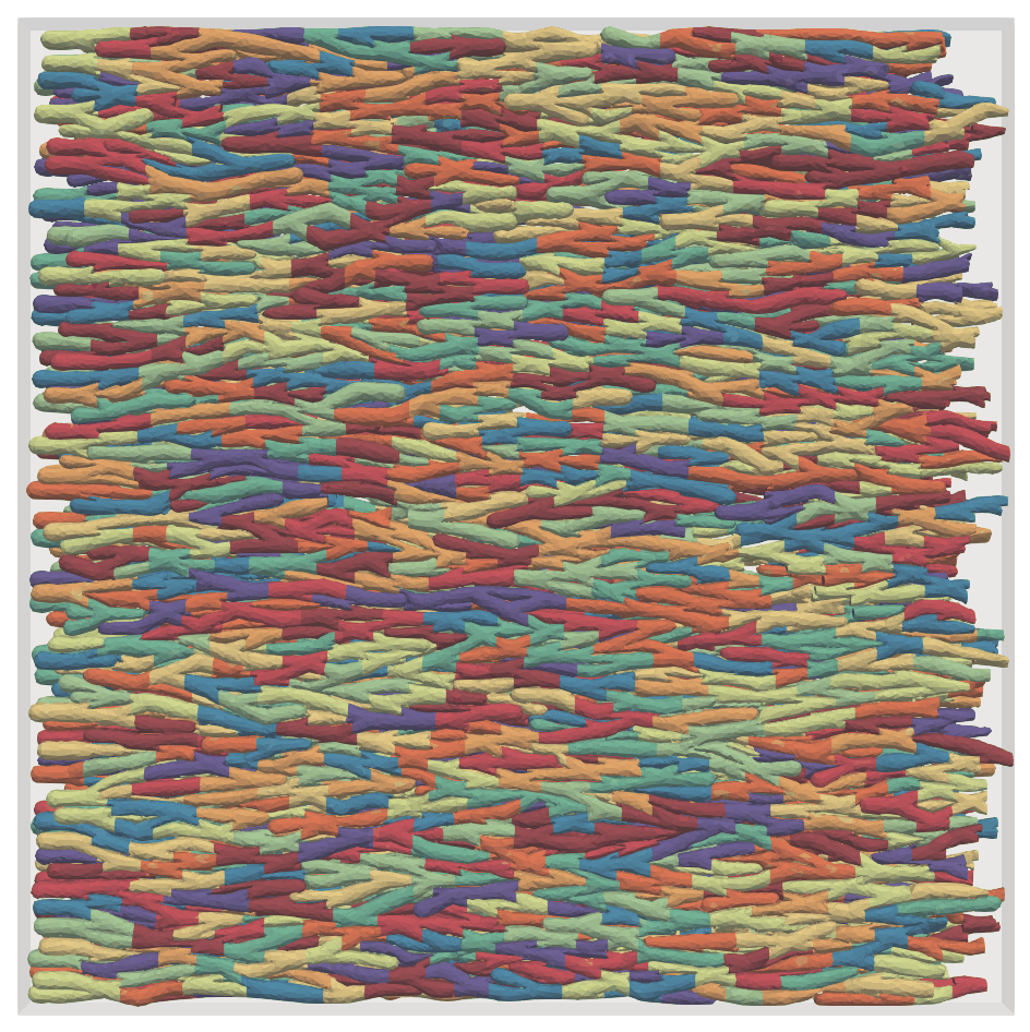
The underlying geometry has been generated with the synthetic mesh generator anni 1 , which has an extent of \(\Omega = (1543 \times 93 \times 1543)\ \mu\mathrm{m}^3\) (the figure below). It resolves 1616 cardiomyocytes, each carrying its own intracellular tag, embedded in a subdivided extracellular domain.
At all intercalated discs (the membranes separating neighbouring cardiac cells), \(\Gamma_\mathrm{g} = \Omega_\mathrm{i}^j \cap \Omega_\mathrm{i}^k\), we assume a simple Ohmic relationship using the Plonsey et al. model 2 :
\[I_\mathrm{g} = \frac{V_\mathrm{g}}{R_\mathrm{g}},\]
where \(I_\mathrm{g}\) and \(V_\mathrm{g}\) are the intercellular current and voltage, respectively and \(R_\mathrm{g}\) denotes the resistance at the intercalated disc. For healthy cardiac cells, we chose the Courtemanche et al. model 3 . We chose an intracellular conductivity of \(\sigma_\mathrm{i} = 0.8\ \mathrm{S/m}\) and an intercellular resistance of \(R_\mathrm{g} = 0.0005\ \mathrm{k\Omega\,cm^2}\) to obtain a longitudinal conduction velocity of approximately \(\mathrm{CV} = 0.86\ \mathrm{m/s}\). Their global specification is given by:
model.ConductivityRegionEMI.intra_default(g_bath=0.8)
model.ionic.PlonseyIonicModel(None, 'default_gap_junction',
                              Rm=0.0005, emi=True)
We define three different domains (spanning over the whole tissue width, i.e. in \(y\) direction):
- a circular scar core with radius \(r\) in the centre of the bounding box of the intracellular cell network \(\Omega_\mathrm{i}\),
- a border zone modelled as a concentric ring around this scar core of width \(w\),
- healthy tissue outside both.
Radius and width are set on the command line via --scar-core-radius and --border-zone-ring-width in microns.
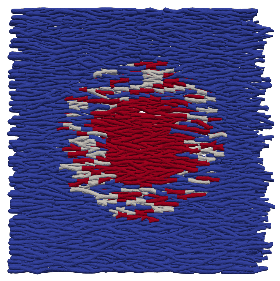
In order to associate each cardiac cell with one of the three regions, the bounding box of each cardiac cell \(\Omega_\mathrm{i}^j\) is first determined. The centres of their bounding boxes then allow for an unambiguous association of a cardiac cell with one of the three regions. The resulting regions are shown in the figure below. The electrophysiology of the different regions is modelled as follows:
| Region | Ionic model(s) | Represents |
|---|---|---|
| Scar core | Plonsey | unexcitable cardiomyocytes throughout |
| Border zone | Courtemanche / Plonsey / MacCannell 4 , equal parts | a mixture of excitable myocytes, unexcitable myocytes and fibroblasts (MacCannell) |
| Healthy tissue | Courtemanche | excitable myocytes |
Note that, since anni is only capable of producing myocyte networks for now, the fibroblasts we model with the MacCannell model have a considerably larger size than actual fibroblasts (by imposing it on cells whose geometry and extent was meant to be for myocytes). Within the border zone the three models are assigned at random in equal thirds, seeded by --seed so that a given parameter set is reproducible.
Ionic models (here, Courtemanche, Plonsey and MacCannell) live on the membranes defining the intersection of intra- and extracellular domains, \(\Gamma_\mathrm{m} = \Omega_\mathrm{i} \cap \Omega_\mathrm{e}\). Since it occupies the largest part of the collection of cardiac cells, we set the Courtemanche model as the default one:
model.ionic.CourtemancheIonicModel(None, 'default_ionic', emi=True)In order to impose an ionic model that differs from that default to a certain cardiac cell \(j\), we need to identify its membrane. The membrane of a cardiac cell in the EMI model is defined by the intersection of its intracellular domain \(\Omega_\mathrm{i}^j\) with the surrounding extracellular domain. In the openCARP implementation of the EMI model, the extracellular domain is subdivided into uniquely-tagged regions (to better distribute the ranks over the extracellular domain, which, if being dealt by only one rank, would occupy most of the compute time). Intracellular and extracellular domains are listed in the .intra and .extra files. In our case, all intracellular domains are given by odd and all extracellular domains by even tags. Thus, for a given cardiac cell \(j\) with an odd tag \(m\), its membrane is defined by tag pairs of \(m\) with the even tags \(n\) of all extracellular subdomains that border that cell. For example, assuming we have one cardiac cell with tag 103, which is surrounded by extracellular subdomains with tags 102 and 104, its membrane is defined by the tag pairs 103:102 and 103:104. These tag pairs need to be determined and explicitly stated for all cardiac cells on which, in this example, another ionic model than the Courtemanche model is imposed. In run.py, this is done in the function region_pairs, which reads the mesh and collects the tag pairs for cardiac cells using the MacCannell and Plonsey model, respectively, and caches it in JSON format. The returned lists are passed straight to the ionic model constructors:
pairs = region_pairs(meshname, args.scar_core_radius,
                     args.border_zone_ring_width, args.seed, CACHE_DIR)

model.ionic.MacCannellIonicModel(pairs['MacCannell'], 'MacCannell', emi=True)
model.ionic.PlonseyIonicModel(pairs['Plonsey'], 'Plonsey',
                              Vrest=-81.2, emi=True)
Cells assigned the Courtemanche model are never listed: they are already covered
by imp_region_emi[0].
Simulation
./run.py --np 72NB: We identified 72 ranks to yield the best runtime on one node. This number may differ, depending on your setup. A PETSc configuration tuned for this problem (hypre_parab_opts) is loaded automatically.
Visualisation
Adding --render renders the resulting spatiotemporal dynamics of the
transmembrane voltage to a series of frames and an mp4 using PyVista (the figure below).
This step is optional and needs pyvista, imageio and imageio-ffmpeg,
which are not part of the openCARP container image; run it in a Python
environment that provides them, or omit --render and visualise vm.igb
with meshalyzer instead:
./run.py --np 72 --render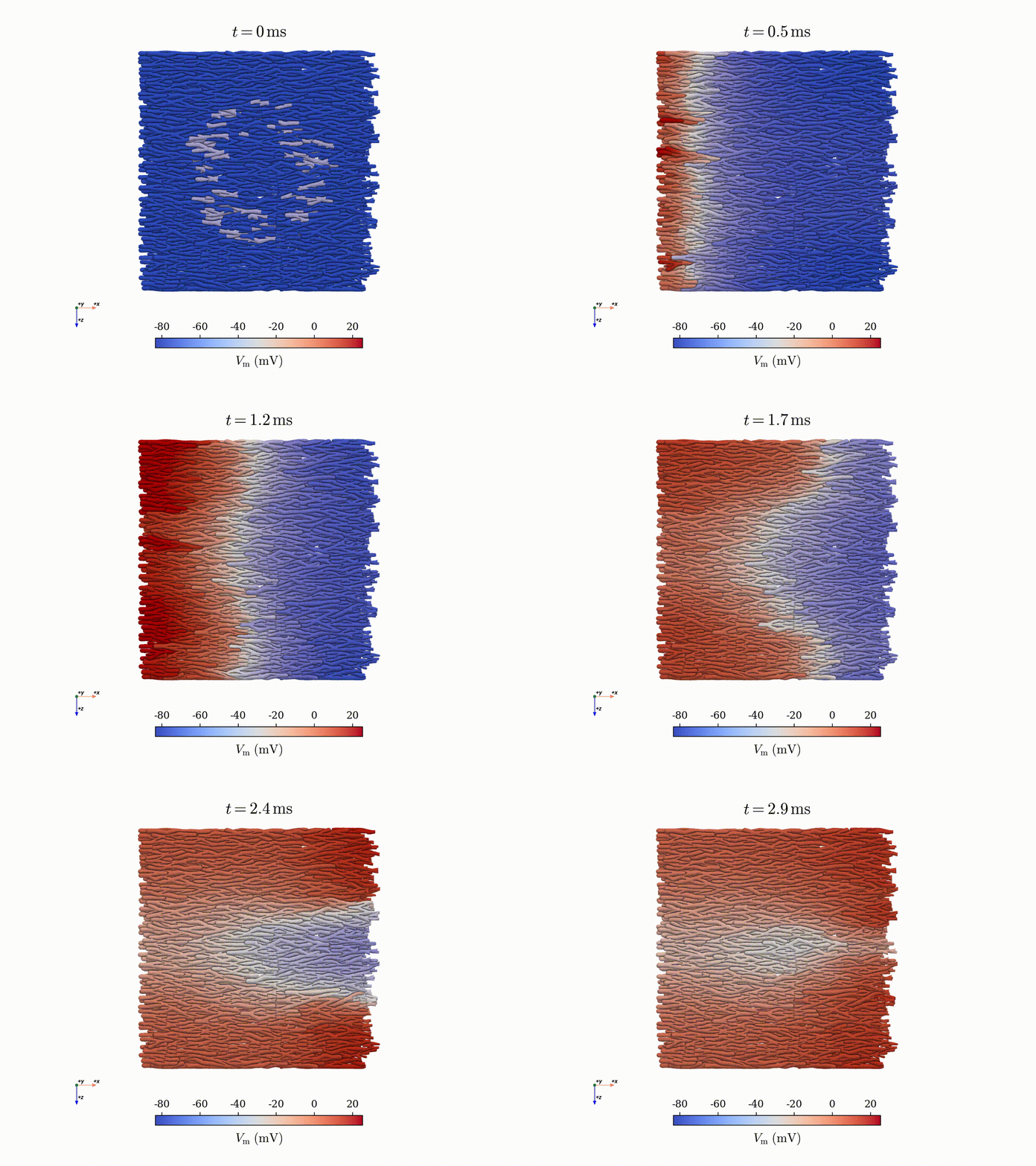
Usage
cd ${EXAMPLES}/07_EMI/02_multi_ionics

# default geometry: 250 µm core, 200 µm border zone
./run.py --np 72 --render

# wider border zone
./run.py --np 72 --border-zone-ring-width 400 --render

# a different random assignment within the border zone
./run.py --np 72 --seed 7 --render
References
Potse, M., Cirrottola, L. & Froehly, A., A practical algorithm to build geometric models of cardiac muscle tissue, 8th European Congress on Computational Methods in Applied Sciences and Engineering (ECCOMAS Congress 2022), 2022. DOI: 10.23967/eccomas.2022.027↩︎
Plonsey, R., The formulation of bioelectric source-field relationships in terms of surface discontinuities, Journal of the Franklin Institute, 297(5), 317-324, 1974. DOI: 10.1016/0016-0032(74)90036-2↩︎
Courtemanche, M., Ramirez, R. J. & Nattel, S., Ionic mechanisms underlying human atrial action potential properties: insights from a mathematical model, American Journal of Physiology, 275(1), H301-H321, 1998. DOI: 10.1152/ajpheart.1998.275.1.H301↩︎
MacCannell, K. A., Bazzazi, H., Chilton, L., Shibukawa, Y., Clark, R. B. & Giles, W. R., A mathematical model of electrotonic interactions between ventricular myocytes and fibroblasts, Biophysical Journal, 92(11), 4121-4132, 2007. DOI: 10.1529/biophysj.106.101410↩︎
Recent questions tagged EMI, carputils, ionic_models, fibrosis
There are tagged with EMI, carputils, ionic_models, fibrosis.
Here we display the 5 most recent questions. You can click on each tag to show all questions for this tag.
You can also ask a new question.