Defining electrodes to stimulate tissue in openCARP
See code in GitLab.
Author: Tobias Gerach tobias.gerach@kit.edu, Jonathan Krauß jonathan.krauss@kit.edu
To run the experiments of this example change directories as follows:
cd ${EXAMPLES}/02_EP_tissue/24_electrode_definitionAnatomy of a stimulus
Every stimulus stim[i] in openCARP is assembled from four independent building blocks.
The circuit crct defines what is applied, the electrode elec where, the protocol
ptcl when, and the pulse pulse how the stimulus evolves over time.
Each block can be changed without touching the others, which is exactly what this example does.

All experiments use the same tissue: a \(10 \times 5 \times 1\) mm slab
(0.2 mm resolution) solved with the bidomain model and the Drouhard-Roberge ionic model with
shortened action potentials, so that repeated stimuli can be demonstrated in a few minutes.
One stimulus called S1 is placed in the center of the slab.
Three command line options select the building blocks,
./run.py --electrode {block,sphere,cylinder,tag,vtx,vtx_fcn} \
         --pulse     {monophasic,biphasic,sine,trc} \
         --protocol  {single,periodic,stimlist}
and --center and --size (both in mm) move and scale the electrode.
Two openCARP options help to check what a stimulus actually does, and every run of this example turns them on:
stim[i].elec.dump_vtx_file = 1writes the nodes selected by the electrode toS1.vtx. Note that this file is written to the directory openCARP was started from, not to the simulation directory.stim[i].pulse.dumpTrace = 1writes the sampled pulse toS1.trcin the simulation directory. The trace is the pulse shape, i.e. before it is multiplied bypulse.strength.
Adding --visualize plots both files, the stimulated nodes and the applied pulse over the
whole protocol, and opens the transmembrane voltage in meshalyzer.
Circuit: what is applied
stim[i].crct.type sets the physics of the source and therefore also the unit of
pulse.strength:
| type | source | unit of pulse.strength |
|---|---|---|
| 0 | transmembrane current | µA/cm² |
| 1 | extracellular current | µA/cm³ |
| 2 | extracellular potential (closed loop) | mV |
| 3 | extracellular ground | (none, enforces 0 mV) |
| 4 | intracellular current | µA/cm³ |
| 5 | extracellular potential (open loop) | mV |
| 6 | illumination | mW/mm² |
| 9 | transmembrane potential clamp | mV |
This example uses transmembrane currents, except for the spatially varying electrode below, which needs a potential. The physics and wiring of extracellular stimuli (grounding, balancing, open and closed loops) are explained in detail in the extracellular stimulation example.
Electrode: where it is applied
openCARP offers three ways to select the stimulated nodes, checked in this order:
- a vertex file
elec.vtx_file, which lists node indices explicitly, - a mesh tag
elec.geomID, which selects all nodes of the elements carrying that tag, - a geometric shape
elec.geom_type, which selects all nodes inside a sphere, block, or cylinder.
If more than one is given, the first one in this list wins. Geometric shapes are the quickest way for simple meshes, tags are the natural choice for anatomical structures that are already labelled in the mesh (e.g. the sinus node), and vertex files give full control.
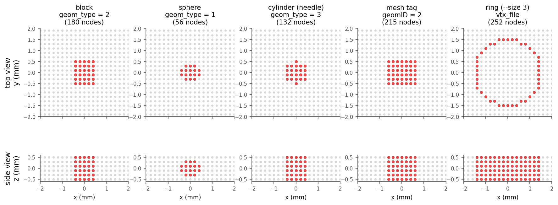
S1.vtx, red). All use the default settings
except the ring, which is shown for --size 3.Geometric shapes
Shapes are described by the points elec.p0, elec.p1 and elec.radius, all in
µm:
geom_type |
shape | parameters |
|---|---|---|
| 1 | sphere | p0 center, radius |
| 2 | block | p0 lower corner, p1 upper corner |
| 3 | cylinder | p0 and p1 ends of the axis, radius |
For a block, openCARP expects p0 to be smaller than p1 in every coordinate, otherwise
the electrode is empty and openCARP aborts with Empty stimulus[0] electrode def.
For a cylinder, p0 and p1 are not corners but the two ends of its axis, and the
cylinder ends flat at both points.
The cylinder in this example is a needle electrode that pierces the slab along \(z\).
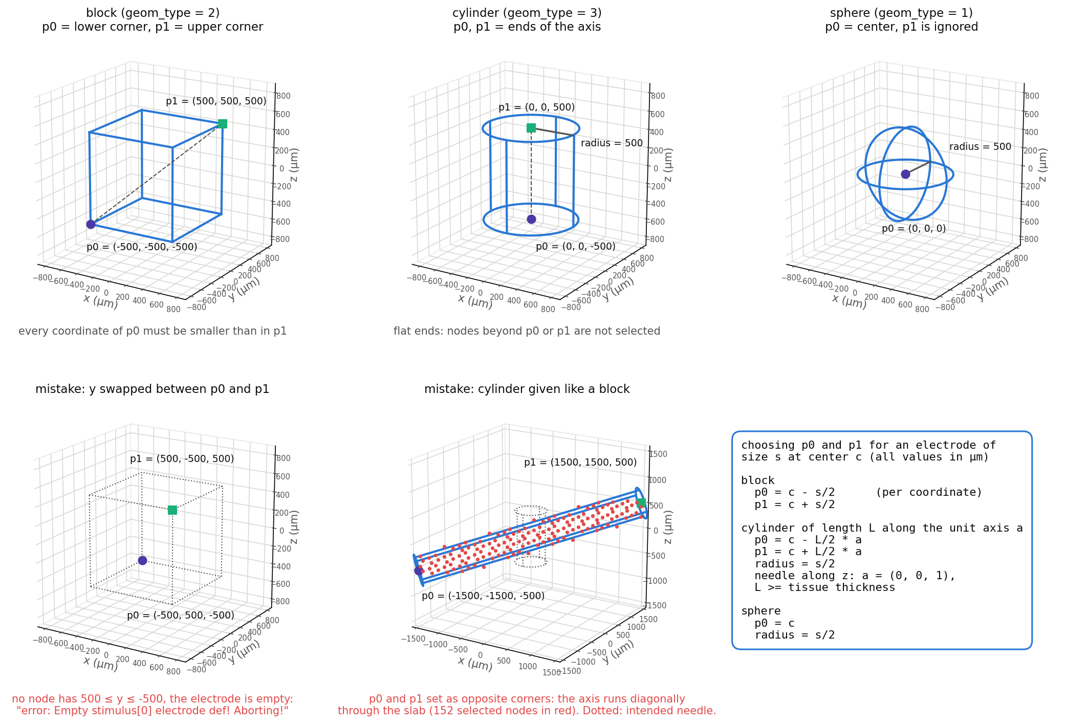
p0, p1 and radius define each shape, with the values this example uses.
Bottom: two common mistakes, run with openCARP. The selected nodes are shown in red.
Bottom right: how to compute p0 and p1 from the electrode center and size../run.py --electrode block --visualize
./run.py --electrode sphere --visualize
./run.py --electrode cylinder --visualizeMesh tags
With --electrode tag the script adds a box shaped region with tag 2 to the mesh and sets
elec.geomID = 2. Compare the dumped nodes with those of the geometric block of the same
size: a tag selects all nodes of the tagged elements, a shape selects the nodes inside the
shape. The tag based electrode is therefore slightly larger, 215 instead of 180 nodes with the
default settings.
./run.py --electrode tag --visualizeVertex files
A vertex file lists the number of nodes, the grid the indices refer to, and one node index per line:
252
extra
278
279
...
The indices always refer to the input mesh, so the second line should read extra even for
intracellular stimuli (openCARP warns if it reads intra).
With --electrode vtx the script writes a ring of nodes around --center to
S1_electrode.vtx, a shape none of the geometric definitions can describe.
With a large enough ring, the two wavefronts it launches, one spreading outwards and one
collapsing inwards, are easy to spot in meshalyzer.
./run.py --electrode vtx --size 3 --visualizeSpatially varying electrodes
Setting elec.vtx_fcn = 1 reads a second column from the vertex file and scales the
stimulus at each node by it:
156
extra
0 0.0000
51 0.0400
...
Warning
The nodal scaling is only applied to potential stimuli (Dirichlet boundary conditions,
e.g. crct.type = 2). For current stimuli it is silently ignored.
With --electrode vtx_fcn the whole left face of the slab becomes an electrode that imposes
an extracellular potential of -2 V scaled linearly from 0 at \(y_{\mathrm{min}}\) to 1 at
\(y_{\mathrm{max}}\). The right face is grounded (crct.type = 3) to provide the reference
potential. The electrode is cathodal (negative) because a positive electrode hyperpolarizes
the tissue beneath it. The tissue is excited first where the scaling is largest.
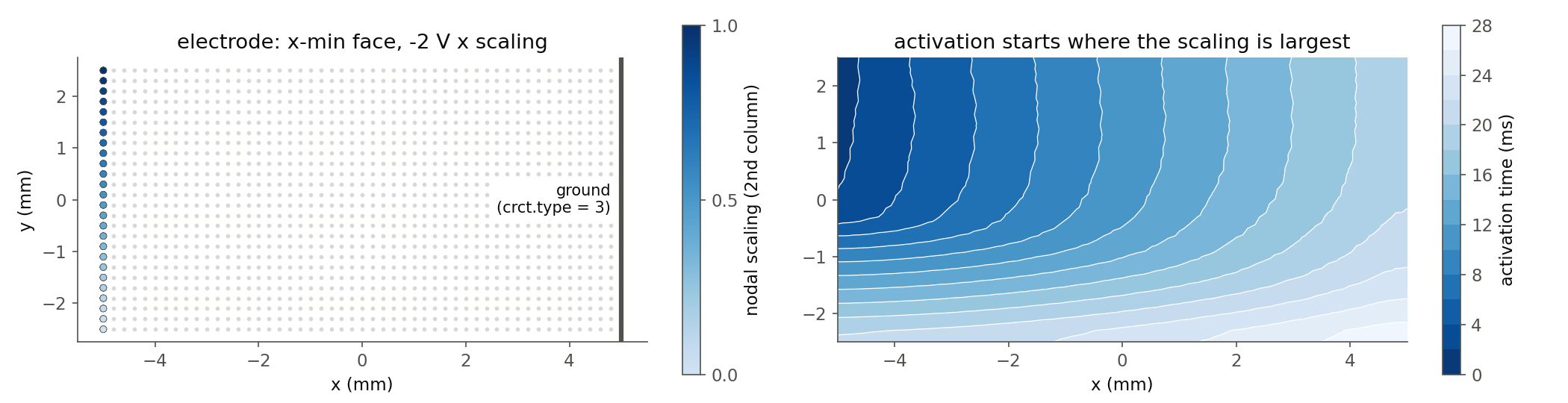
./run.py --electrode vtx_fcn --visualizeProtocol: when it is applied
The protocol stim[i].ptcl sets the timing of the stimulus:
ptcl.startandptcl.durationdefine a single stimulus,ptcl.nplsandptcl.bclrepeat itnplstimes with a basic cycle lengthbcl,ptcl.stimlistgives arbitrary onsets as a comma separated list. An entry starting with+is relative to the previous onset, so"1,+150,+200"equals"1,151,351".nplsandbclare ignored when a stimlist is given.
ptcl.duration is the length of one stimulus and must be shorter than bcl.
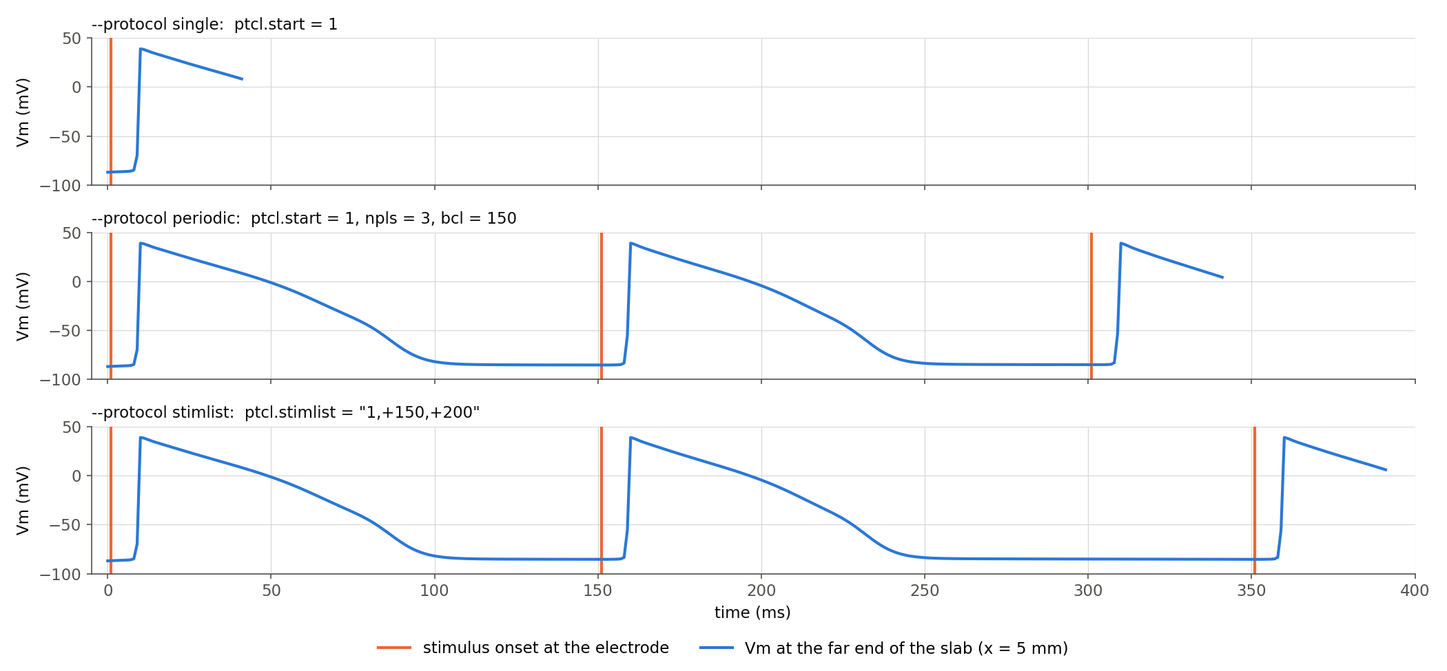
./run.py --protocol single --visualize
./run.py --protocol periodic --visualize
./run.py --protocol stimlist --visualize
Pulse: how it looks over time
stim[i].pulse.strength sets the amplitude, the unit follows from crct.type.
stim[i].pulse.shape selects a built-in waveform:
0: square wave, a step atpulse.trigthat lasts until the end ofptcl.duration,1(default): truncated exponential. With its default time constantstau_edgeandtau_plateauit is practically a square pulse. Settingpulse.d1 < 1makes it biphasic, whered1is the relative duration of the first phase ands2the relative strength of the second phase with inverted polarity,2: sine wave with frequencypulse.freq(in cycles per ms) and phasepulse.phase.
Any other waveform can be read from a trace file with pulse.file (see below).
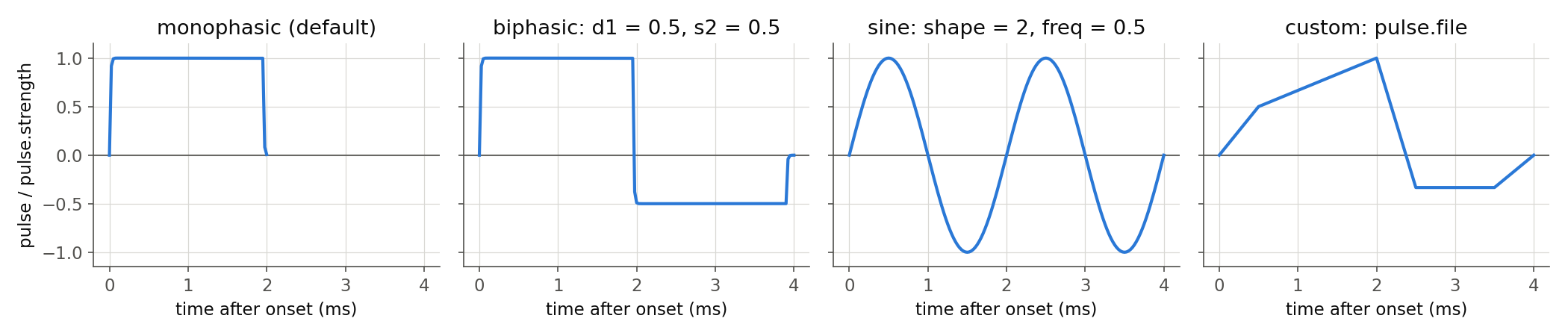
--pulse monophasic, biphasic, sine and trc as written
by pulse.dumpTrace../run.py --pulse monophasic --visualize
./run.py --pulse biphasic --visualize
./run.py --pulse sine --visualize
./run.py --pulse trc --visualizeThe activation times written by this example detect every upstroke (lats[0].all = 1).
Biphasic and sine pulses drive the transmembrane voltage inside the electrode below and above
the detection threshold, so a few electrode nodes report more than one activation. These are
stimulus artifacts, not additional beats.
Trace files
A trace file (extension .trc) starts with the number of samples, followed by one pair of
time (ms, relative to the stimulus onset) and value per line.
Time steps do not have to be equidistant, but must increase.
The .trc extension in pulse.file is optional.
openCARP processes the file in three steps:
- The values are divided by their largest magnitude, so only the shape matters and the file can use any unit.
- The result is multiplied by
pulse.strength. - It is linearly interpolated onto the time step for the duration
ptcl.duration. Ifptcl.durationis longer than the trace, the last value is held. If it is shorter, the trace is cut.
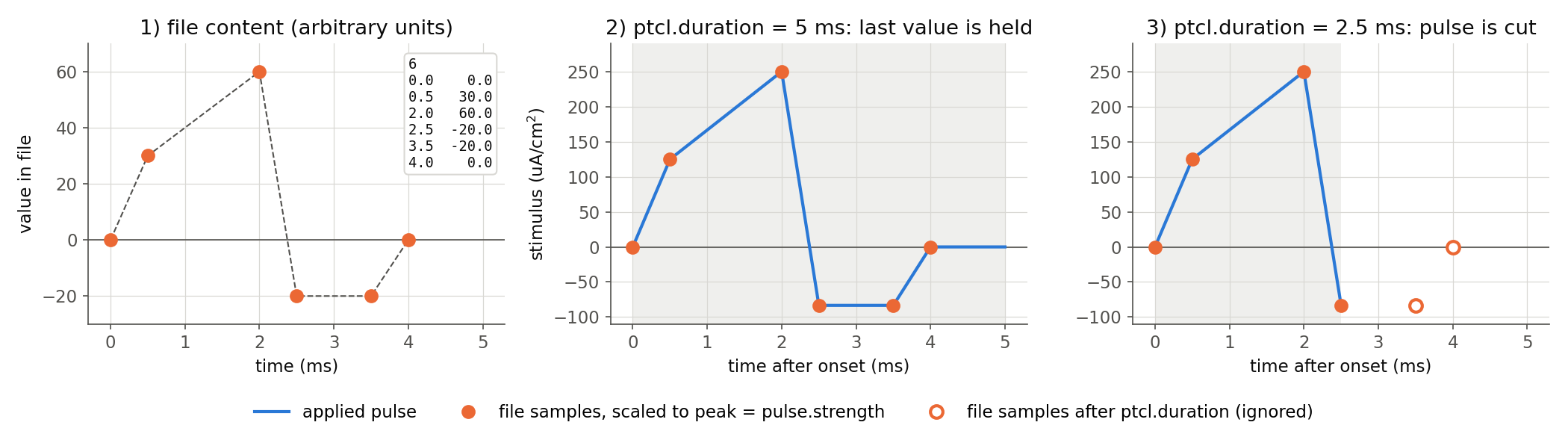
--pulse trc (left) and the applied pulse for two different values of
ptcl.duration with pulse.strength = 250.Because the protocol repeats the full pulse for every onset, a trace file only needs to describe a single stimulus, not the whole basic cycle length.
Recent questions tagged experiments, examples, stimulus, tissue, electrode, vtx, trace, protocol
There are tagged with experiments, examples, stimulus, tissue, electrode, vtx, trace, protocol.
Here we display the 5 most recent questions. You can click on each tag to show all questions for this tag.
You can also ask a new question.